Strange Attractors (12 Months of aRt, February)
February 28, 2019
What is a strange attractor?
Wikipedia says an attractor is a set of numbers towards which a system tends to evolve. It then says that an attractor is called strange if its set is fractal. If you’re like me, that definition went in one ear and out the other. Here’s an infinitely better definition:
Imagine how a planet orbits a star. The planet is attracted to the center of the star by gravity, but its angular momentum flings it into an ellipse, rather than just letting it fall towards the star. If we took an orbiting planet and traced its path over many cycles of revolution around the star you would see a pattern of overlapping ellipses. But what if the point of attraction (the star in our example) was not a point? What if it was a line? Or a curve? Or any other function we can define mathematically? Imagine what the orbital path would look like if a star was shaped like a cylinder instead of a sphere. As the planet orbited, it would not experience a uniform gravitational pull at each point in its revolution; it would experience more gravitational attraction as it approached the poles of the cylinder, which would in turn affect its momentum and create a very different path than before. A strange attractor is a system just like the planet and star, except that the “point” of attraction is not a simple point or line, but a complex mathematical function with discontinuities. We draw pictures by releasing a particle (our planet) and then following its path as it orbits our discontinuous attractor function (our star). Because the attractive force on the particle is not continuous, it will be highly sensitive to whatever the precise state of the system at each timepoint, and will often form complex patterns that seem random, but eventually form a repeating orbit.
What does this actually look like mathematically? First we define a starting point for our particle in (x_0, y_0) coordinates—often (0, 0). Then we use this as input for an attractor function that defines what the next value (x_1, y_1) will look like. Here’s an example attractor function: x_n = sin(a*y_{n-1}) + c*cos(a*x_{n-1}) y_n = sin(b*x_{n-1}) + d*cos(b*y_{n-1})
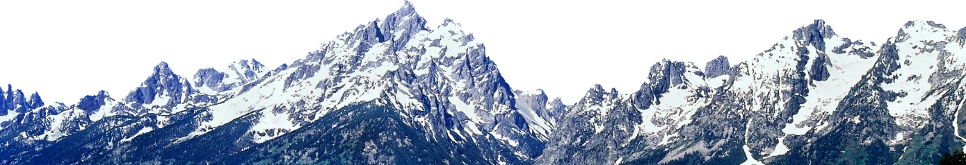
We loop through this function, using the previous particle position as input until we have many points. In these equations, a, b, c, d are constants that we can change to obtain a different looking attractor. The above function with parameters a = 1.24, b = -1.25, c = -1.81, d = -1.91, and 10 million points produces this picture.
Inspiration
My first exposure to strange attractors in R came from this blog post by Antonio Chinchón. Antonio very cleverly used Rcpp to calculate the position of each point in the attractor. Around the same time, I saw the incredible work on the blog Softology about all different types of strange attractors. So with Rcpp implementation in hand and a whole mess of attractors to try, I strode forward, copying & pasting my way to success until I got something to form on my screen. But I would never be satisfied just copying an attractor formula and tweaking some parameters, so I started digging into the formula to see what I could make.
How to make attractors in R
My first attempts at making attractors used the Rcpp implementation of Antonio Chinchón. Here we define the start points and constants, then use them as input for an Rcpp loop where we have our attractor functions. This makes an output dataframe with the x and y coordinates of our points, which we then plot using ggplot. That code looks like this:
library(Rcpp)
library(ggplot2)

#an attractor of my own devising

#ggplot theme blank canvas
opt = theme(legend.position  = “none”,
            panel.background = element_rect(fill=”white”),
            axis.ticks       = element_blank(),
            panel.grid       = element_blank(),
            axis.title       = element_blank(),
            axis.text        = element_blank())

#Rcpp attractor function
cppFunction(‘DataFrame createTrajectory(int n, double x0, double y0,
            double a, double b, double c, double d) {
            // create the columns
            NumericVector x(n);
            NumericVector y(n);
            x[0]=x0;
            y[0]=y0;
            for(int i = 1; i < n; ++i) {
            x[i] = sin(a*y[i-1])*sin(a*y[i-1])+c*cos(a*x[i-1])*cos(a*x[i-1]);
            y[i] = sin(b*x[i-1])*sin(b*x[i-1])+d*cos(b*y[i-1])*cos(a*x[i-1]);
            }
            // return a new data frame
            return DataFrame::create(_["x"]= x, _["y"]= y);
            }
            ')

#define constants
a=-2
b=1
c=0.5
d=-0.9

#make dataframe and plot the points
df=createTrajectory(5000000, 0, 0, a, b, c, d)
ggplot(df, aes(x, y)) + geom_point(color="#1E1E1E", shape=46, alpha=.01) + opt
Rcpp is used because the typical way to make these points is by defining your attractor function and starting position of the particle, then calculating the new x and y coordinates of the particle for millions of generations. This is done as a for-loop, adding new data rowwise. But growing a large dataframe rowwise is generally not a good idea in R for similar reasons as outlined in this blog post. I do not know c++, but I stumbled through it and was able to tweak the simple equations enough in many cases. Eventually, I wanted to define really weird functions with lots of powers, logs, and absolute values. I got stuck with the c++ implementation there (I know, I know… kinda pathetic, but give me a break, I’m a microbiologist by training).
I moved on to trying a pure R implementation. It’s a common misconception that for-loops are categorically slow in R. In our case, if you try to “grow” the dataframe, it will be quite slow. But by pre-initializing vectors of the length you want and then filling them with values, the speed difference with R and Rcpp is barely noticeable. While Rcpp is a few seconds faster in generating the points, it also takes a few seconds to define the Rcpp function, so in the end I found both implementations to be the same speed. And in any case, the plotting takes about 60x longer than calculating the points, so I’m fine if my R solution is half a second slower than Rcpp.
library(ggplot2)
library(dplyr)

#a hopalong attractor

#ggplot theme blank canvas
opt = theme(legend.position  = “none”,
            panel.background = element_rect(fill=”white”),
            axis.ticks       = element_blank(),
            panel.grid       = element_blank(),
            axis.title       = element_blank(),
            axis.text        = element_blank())


#attractor function
createTrajectory <- function(n, x0, y0, a, b, c) {
  #pre-initialize vectors of length n
  x <- vector(mode = "numeric", length = n)
  y <- vector(mode = "numeric", length = n)

  #starting values
  x[1] <- x0
  y[1] <- y0

  #fill vectors with values
  for(i in 2:n) {
    x[i] <- y[i-1]-1-sqrt(abs(b*x[i-1]-c))*sign(x[i-1]-1)
    y[i] <- a-x[i-1]-1
  }

  #make dataframe
  data.frame(x = x, y = y)
}

#constants
a=2
b=1
c=8
v=3

#calculate positions and plot
df=createTrajectory(3000000, 0, 0, a, b, c)
ggplot(df, aes(x, y)) + geom_point(color="#1E1E1E", shape=46, alpha=.05) + opt
Strange attractor sandbox
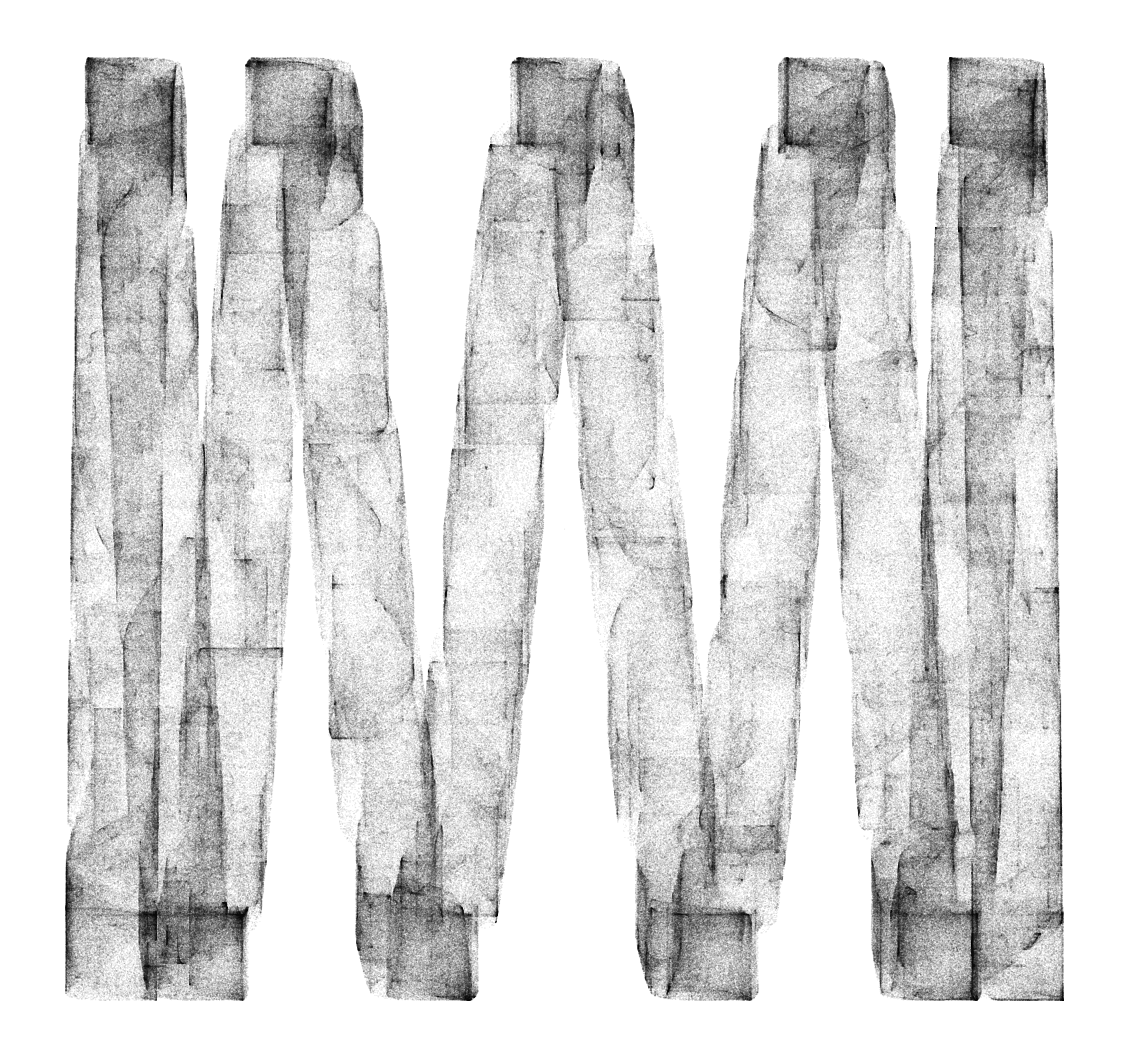
I quickly got bored of the pre-defined attractors, and started just changing the formulas in a more or less random way. In most cases I began with an attractor I knew would work like Clifford or Hopalong, but then quickly altered the formula and kept messing with it until the resulting attractor had very little resemblance to the original. Here are my sketches organized by the general type of attractor I started with or grouped the results into:
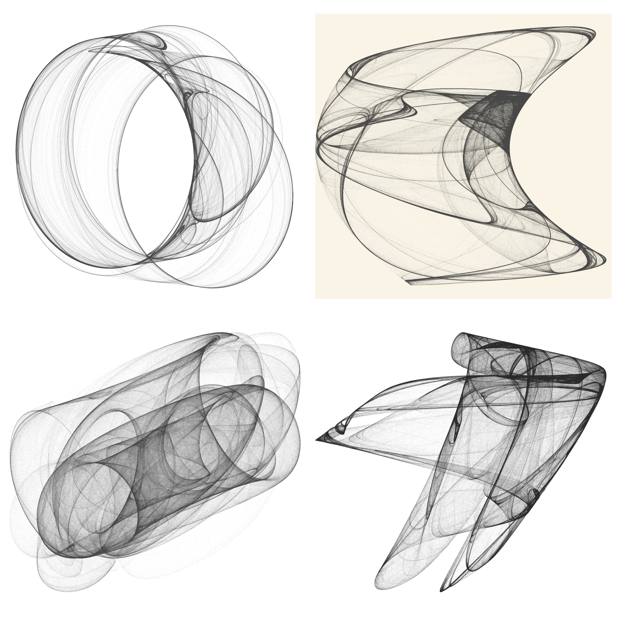
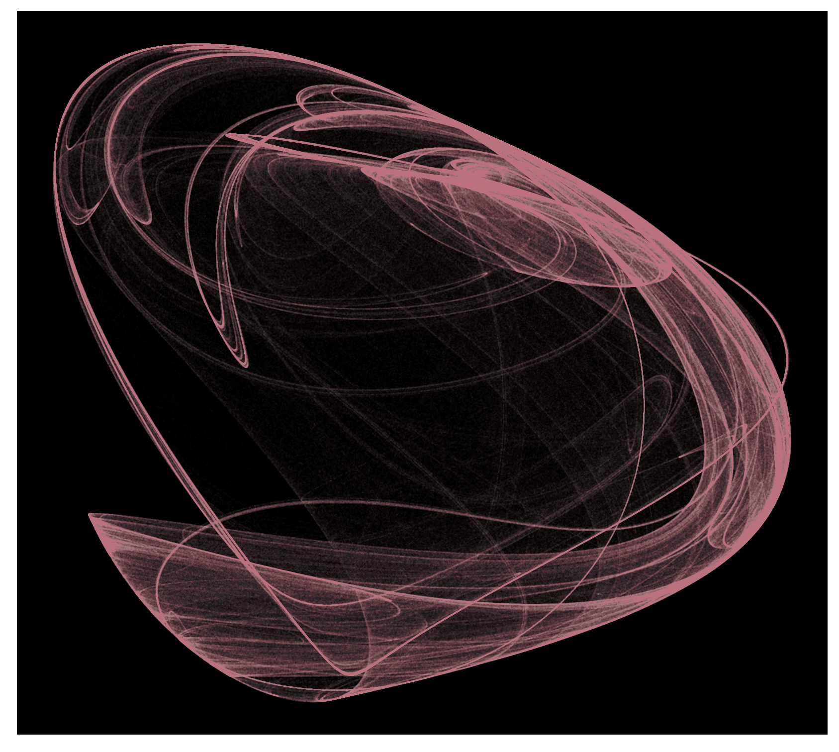
Chase
One of the first things I started changing was the formula of typical Clifford/Pickover/Bedhead attractors. These attractors usually have some combination of sine/cosine functions with constant multipliers. So I just started testing random things: What if I move the constants around? What if I change pluses to minuses? What if I square some of the trig functions? This resulted in a whole set of new attractors that I call “Chase” attractors because I’m not creative with names. I’ve made many different formulas, but have not tested many parameters, so there’s lots to explore in here.
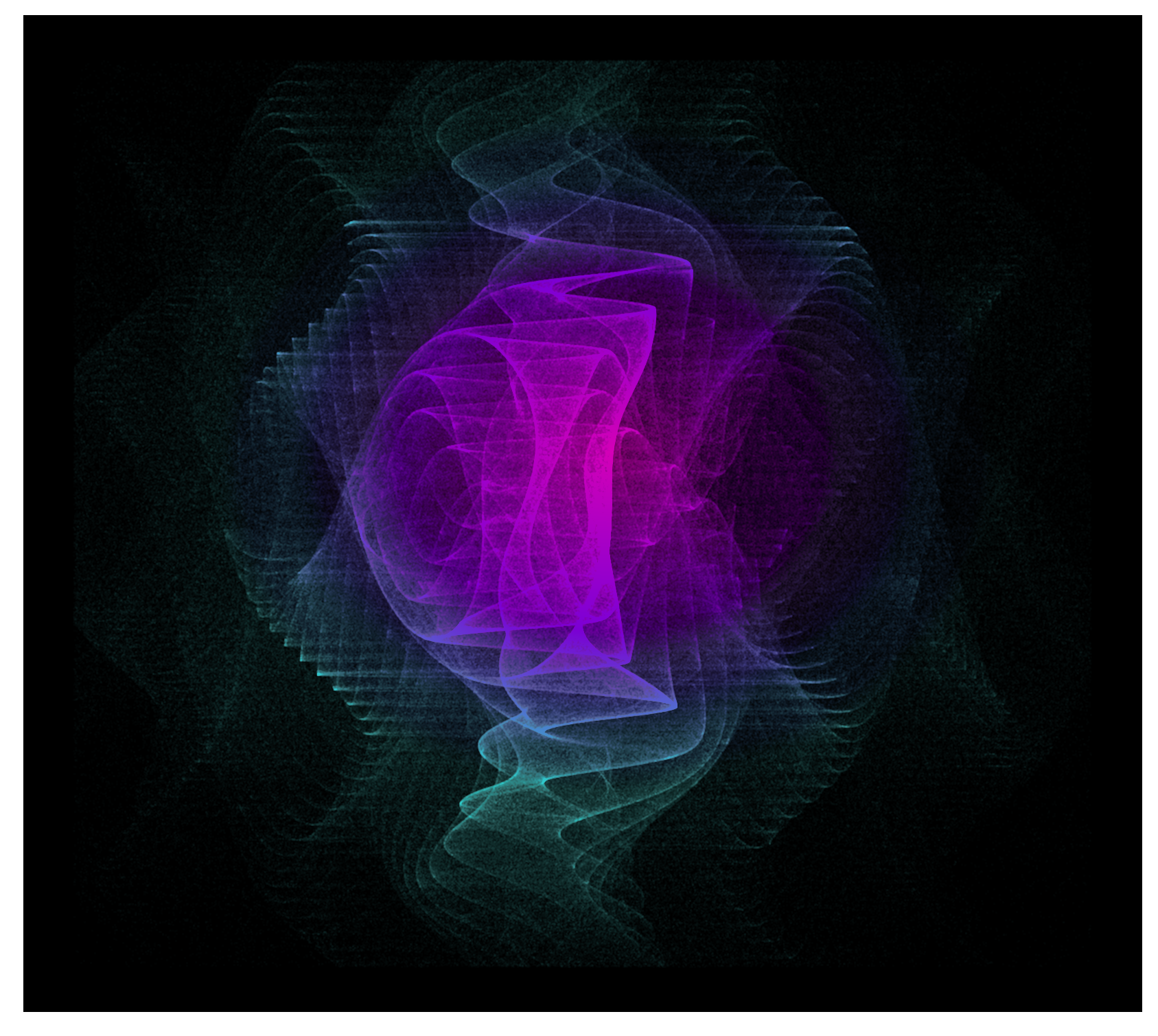
“Ratchet” attractors
From Masaru Fuji I got the idea to add a “ratchet” parameter to attractors. His idea is to add a third function to the attractor function that defines t_n = t_{n-1} + v where v is some constant. Then we can use t_n in our x and y attractor functions. This is probably best thought of as adding a time dimension to the function, but in my head, I think of it like a ratchet wheel, that clicks up one notch for each generation, so I call it a “ratchet” attractor. An interesting property of these attractors is that they are not orbital in the same way as a typical strange attractor. Because of the ratchet parameter, the points will never converge on a stable orbit, so if you plot more points you will keep getting different images. I implemented this idea in many of my subsequent attractors. Here’s what happens if you add this ratchet parameter to my “Chase” attractor, or use it in a modified Clifford attractor.
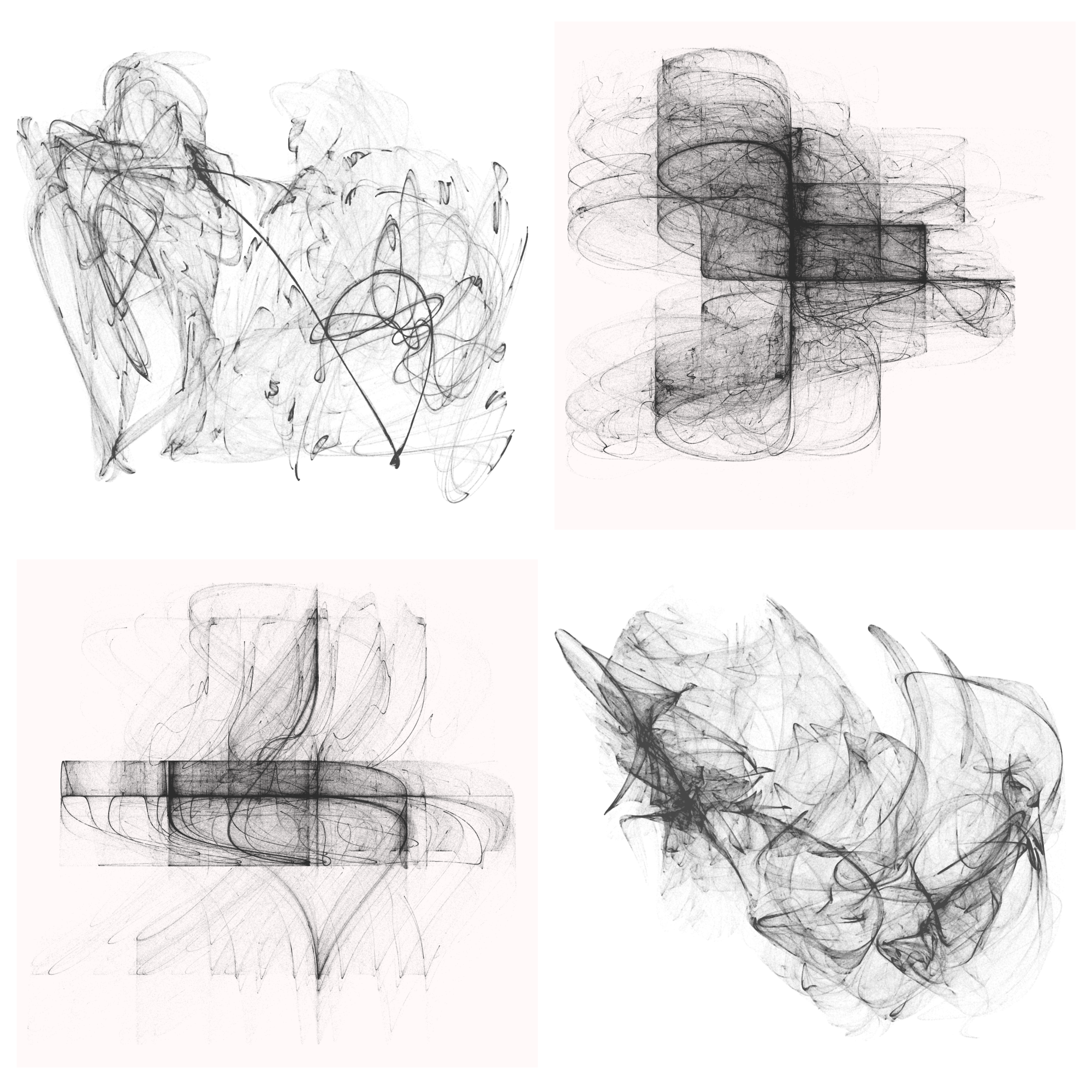
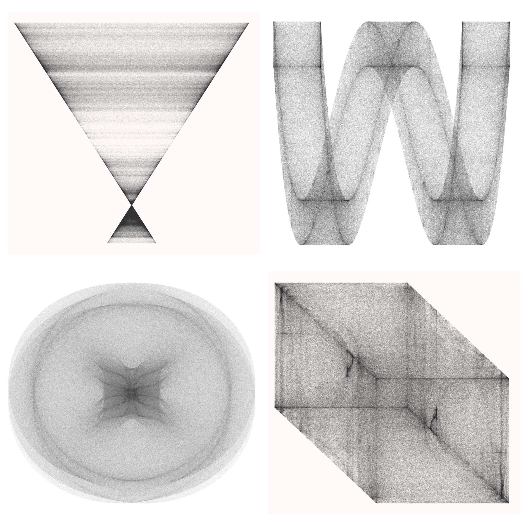
Hopalong attractor
I tried a Hopalong attractor, described here. In this collage, the first image is a standard formula for a Hopalong attractor with no tinkering. The next three are me messing with the formula to get increasingly weird images…
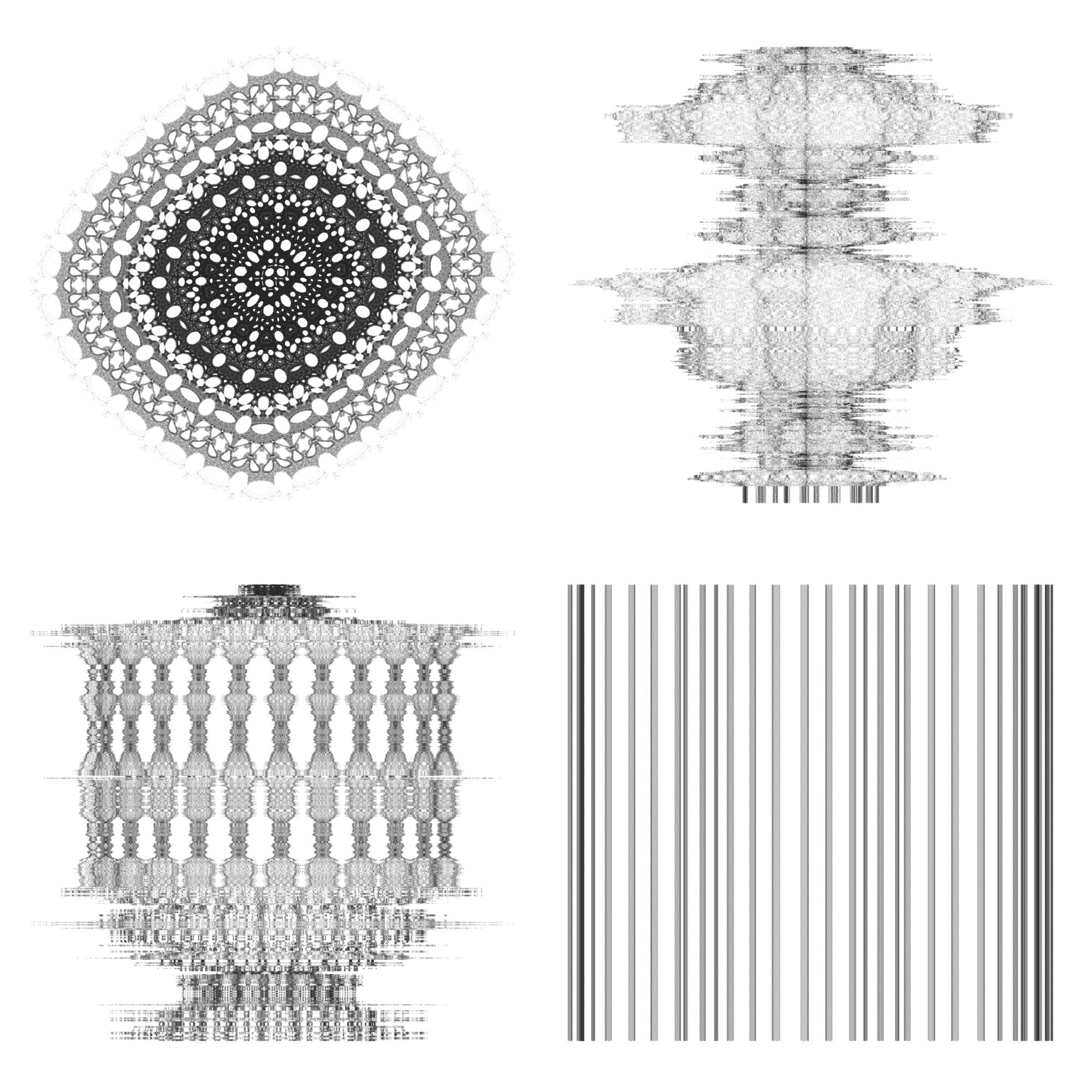
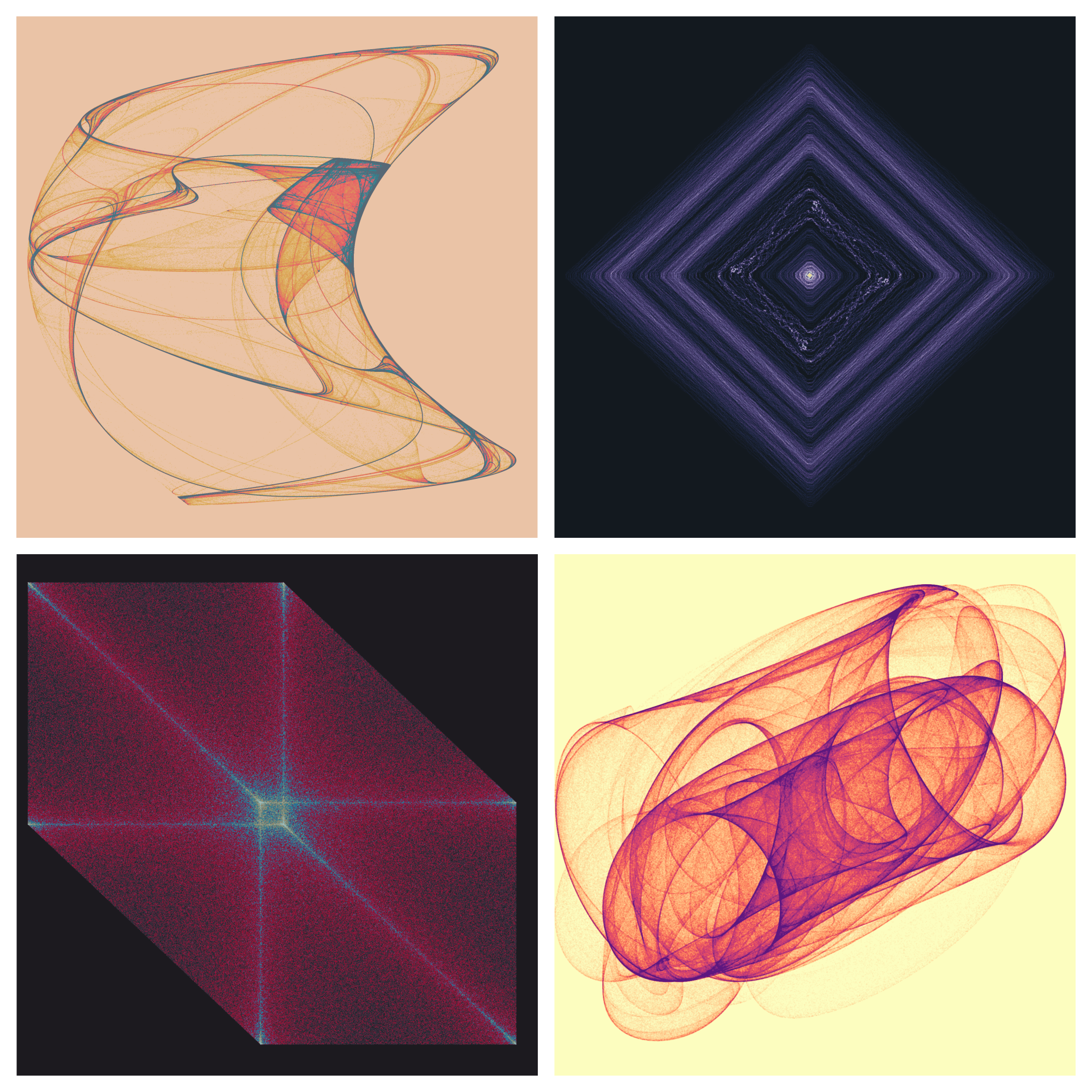
Quadrup-two attractor
For this set I started with a quadup-two orbital map but never actually made anything “normal”. All of these images have altered formulas, but they’re some of my favorites… so weird!
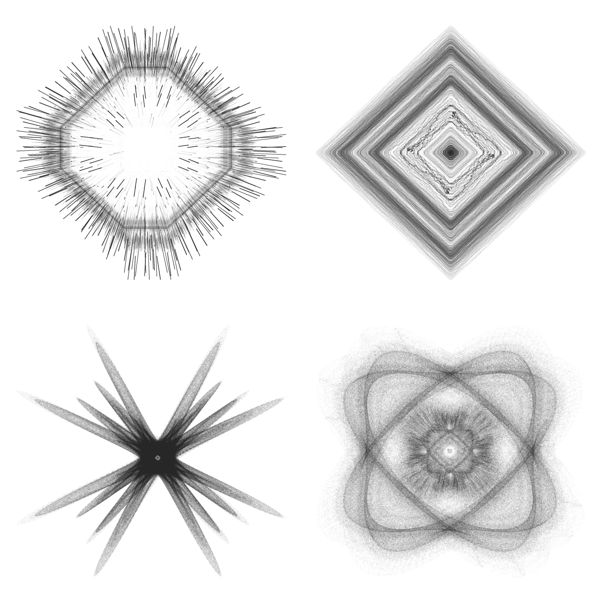
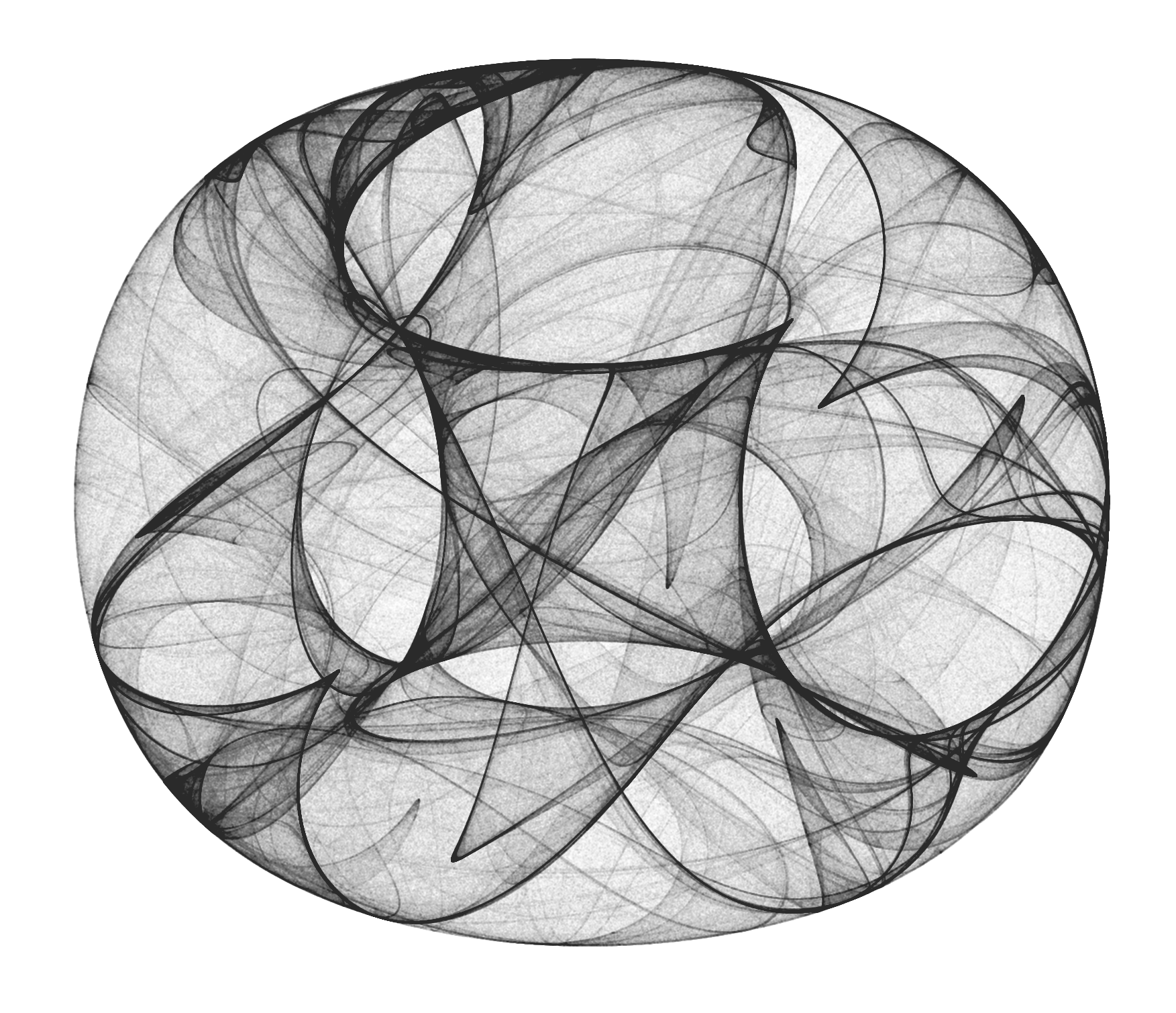
Symmetric attractors
You may have noticed that many of the attractors I’ve shown are roughly symmetric, or they don’t have the typical wavy pattern of other strange attractors you might have seen on the web. I honestly can’t say why this is. I just seem to have a knack for stumbling upon attractors that have very symmetric or geometric shapes. Here’s some more that I happened upon in my tinkering.
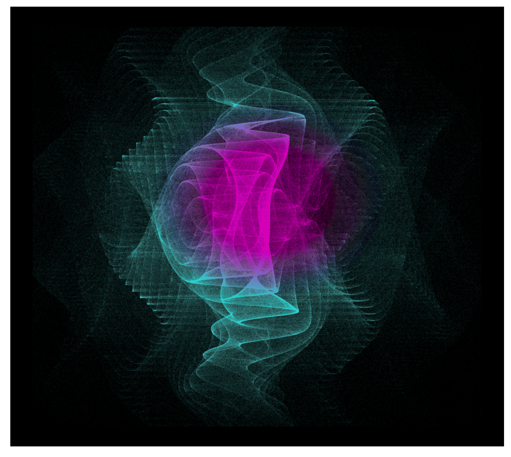
Adding color
I usually go for a black and white start on all of these, and think that many look best in this minimalistic way. But sometimes adding color really lifts an attractor from meh to Wow!… plus color is fun and pretty! There’re many ways to add color: for starters you can just make the points colored and this will give a roughly uniform appearance across the plot.
Another approach is to define some function based on the position of the points. You could also apply a color based on the order of the points. Here’s an example where I calculated the distance from the origin for each point and applied a color ramp based on that distance.
But the most common way to color attractors is based on the density of points at each pixel. Since attractors form orbits, the particle often moves through the same point many times. This is why even though we plot the points with a very high transparency they appear dark in many places. We can use this property to apply a color ramp palette where each pixel is colored by the number of points occupying it. To do this we read in the already rendered black and white image, then use EBImage::colormap to apply some color palette.
library(EBImage)
library(tidyverse)

#read in the image and convert to greyscale
img <- readImage("chase_6.png")
gray <- channel(img, "gray")

#map the color palette to the image
img_col <- colormap(gray, viridis::magma(256))
display(img_col, method = "raster")

#when you are satisfied with the image, save it
writeImage(img_col, "chase_6_color.png")
This technique can produce some very nice images after playing with the palettes a bit.
Your turn!
One takeaway I hope you get from this project is that you don’t need any particular math or programming expertise to make beautiful images with strange attractors. As always, all of my code is on my GitHub, and I highly encourage you to go and try out your own attractors. There’s so much possibility and it really just requires playfulness and patience.
As you define your own attractor functions it’s impossible for someone without a math degree to understand exactly what caused a pattern. There are many attractors already defined that will work, but as you start playing with the formula you will notice that some attractors converge on a single point and do not form a pattern, while others spread out so much that it is just fuzz. Don’t be discouraged… try lots of different parameters, different formulas, different color schemes.
I have two pieces of advice when trying out strange attractors:
1) Sometimes you need to crop the image to make a really compelling picture. By “zooming in” you can see patterns in what might have looked like a rather squished or failed attractor. You can “zoom” in R by doing something like this.
#calculate points with createTrajectory function like normal
#then clip outer points
xmax <- max(df$x)/2.5
xmin <- min(df$x)/2.5
ymax <- max(df$y)/2.5
ymin <- min(df$y)/2.5

df_clip <- df %>%
  filter(x > xmin & x < xmax) %>%
  filter(y > ymin & y < ymax)

#plot
ggplot(df_clip, aes(x, y)) + geom_point(color=”#1E1E1E”, shape=46, alpha=.05) + opt
2) Have no fear! Nothing terrible will happen if your attractor doesn’t work. Made something interesting? Great, now see what happens if you make a parameter 100, or 20000, or if you make it negative, or make it 0.0001. Often the most compelling results come from entirely unexpected changes.