Custom fonts and plot quality with ggplot on Windows

May 6, 2019

Graphics devices are weird, and operating systems are even weirder. If you are a Mac of Linux user, lucky you, you can go on your merry way! But if you’re a Windows user and you’ve ever screamed at your computer “Why the #&*$ wont my fonts work!?!?” or “Why are my plots so &#**ing pixelated!?!”, then read on.

Problem 1: Pixelated graphics

In R, the graphics device used in the plots pane of Rstudio depends on your operating system. Windows uses the eponymous windows graphics device… it sucks. If you’ve ever wondered why your plots look like they came out of a printer from 1995, this is the reason.

The bad news is, I don’t have a fix for the Rstudio plots pane; the good news is I do have a fix for saving your plots without pixelation, and apparently the R/Rstudio team is considering a fix for the plots pane. If you’re exporting your plots as PDFs, you won’t have any issues with pixelation, but if you want to export an image, you will. The reason is that the windows graphics device doesn’t implement anti-aliasing. We can change this by setting the type argument of the png device to "cairo", which does implement anti-aliasing. Note that this requires you have the Cairo package installed.

library(ggplot2)

ggplot(mtcars) +
  geom_violin(aes(x = cyl, y = mpg, group = cyl), size = 2)

#the default behavior will produce a pixelated image
ggsave("pixelated_plot.png")

#this will produce a nice smoothed image
ggsave("beautiful_plot.png", device = "png", type = "cairo")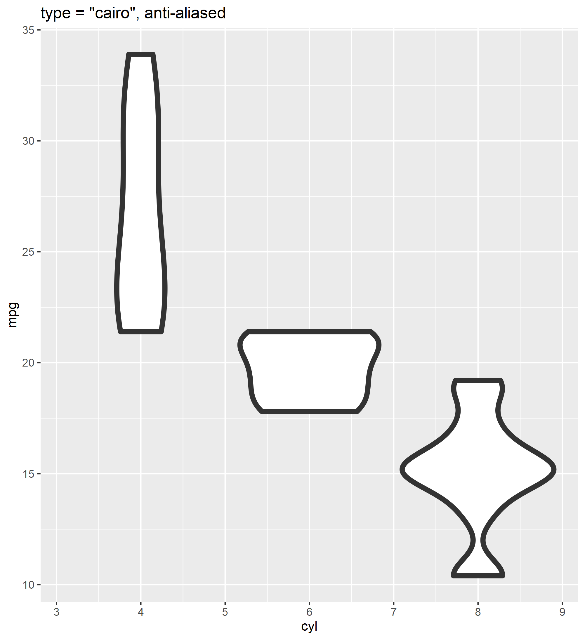

Problem 2: Custom fonts

ggplot2 is built on top of grid. grid does a lot of things well, but text is not one of them. Text, and fonts especially, are a tough problem in graphics libraries, especially given the quirks of how different operating systems work with them. A few packages have popped up for dealing with fonts in R, but the most popular is extrafont. This library works very well, but there are some tricks to getting it to work on Windows that are not easy to find, and beware a lot of the information I’ve seen on StackOverflow is just wrong. Here’s how to load and use custom fonts in ggplot on Windows:

Install the fonts to your system, you can get them from Google fonts or anywhere else
Install the extrafont and extrafontdb packages
Import the fonts to R with extrafont::font_import(), this only needs to be done once or whenever you have installed a new font to your machine
Restart your R session
Load the fonts with extrafont::loadfonts(device = "win"), this has to be done BEFORE you load the ggplot2 package, and it must be done every time you start your R session

This is important, so let me say it again: you have to call extrafont::loadfonts(device = "win") __ BEFORE __ you load ggplot2. A good solution is to add this to your .Rprofile so that it automatically runs every time to start a new R session. Also remember that any time you install a new font, you have to import it to R with extrafont::font_import() before it will be useable. To see which fonts are available for use, you can use extrafont::fonts().

Showing off

Let’s use what we’ve learned to make a quick graph using the Week 19 Tidy Tuesday dataset for 2019. This data is on student-to-teacher ratios around the world. I’ll make a beeswarm plot for each education level colored by continent. I’ll use the Comfortaa font and save the output using the png device with type = "cairo".

#I've downloaded and installed the "Comfortaa" font on my machine
#I've also imported the font to R with extrafont::font_import()

extrafont::loadfonts(device="win")
library(tidyverse)
library(countrycode)
library(ggbeeswarm)

#get data
student_ratio <- readr::read_csv("https://raw.githubusercontent.com/rfordatascience/tidytuesday/master/data/2019/2019-05-07/student_teacher_ratio.csv")

#get country codes + continents information
codes <-
  codelist %>%
  select(iso3c, country.name.en, region, continent)

#calculate summary statistics for each indicator and country
data_summary <-
  student_ratio %>%
  group_by(indicator, country_code) %>%
  summarize(mean = mean(student_ratio, na.rm = TRUE), median = median(student_ratio, na.rm = TRUE)) %>%
  left_join(., codes, by = c("country_code" = "iso3c")) %>%
  filter(!is.na(continent)) %>%
  filter(median < 75) ##note some outliers were removed for aesthetics

data_summary$indicator <- fct_relevel(data_summary$indicator, "Tertiary Education", "Post-Secondary Non-Tertiary Education",
                                      "Upper Secondary Education", "Secondary Education", "Lower Secondary Education",
                                      "Primary Education", "Pre-Primary Education"
                                      )

#plot, notice the base_family argument sets our custom font "Comfortaa"
ggplot(data_summary) +
  geom_quasirandom(aes(x = indicator, y = median, color = continent), size = 2.5) +
  coord_flip() +
  scale_color_manual("Continent", values = c("#E96149", "#B6B800", "#5B9F90", "#DDB089", "#F0C73B")) +
  theme_minimal(base_family = "Comfortaa", base_size = 14) +
  guides(colour = guide_legend(override.aes = list(size=5))) +
  labs(y = "Student to teacher ratio\n(lower = fewer students/teacher)", x = "",
       title = "Student to teacher ratios for world countries, 2012 - 2016",
       subtitle = "Less prosperous countries have more students and fewer teachers",
       caption = "Graphic: @W_R_Chase\nData: UNESCO") +
  theme(plot.background = element_rect(fill = "#F6FCF8"),
        panel.grid.major.y = element_blank(),
        panel.grid.minor.y = element_blank(),
        plot.subtitle = element_text(face = "italic", size = 14),
        plot.title = element_text(size = 18),
        plot.caption = element_text(face = "italic", size = 8, vjust = 0.5, hjust = 1),
        axis.title.x = element_text(margin = margin(t = 20)))

ggsave("tidytuesday_wk19_student_ratios.png", device = "png", type = "cairo", height = 10, width = 12)

Notice our fonts rendered with no issues, and our plot does not show any pixelation. Importantly, this script won’t work if you try to run it verbatim on a Mac or Linux machine, and this is one of the most frustrating parts of this whole mess. There are some fancy things you could try with your .Rprofile and detecting OS, but honestly I haven’t found a solution that I really love yet.