Textures and geometric shapes (12 Months of aRt, July)

July 29, 2019

Motivation

R (the coding language, R) is my happy place, but there’s always been one thing that’s really irked me: the real lack of support for complex fills, filters, or other graphics effects goodness. In R, there’s basically only support for perfectly rendered shapes and solid fills. If you want something like a gradient fill, blur, or texture, you’re left to your lonesome. I really felt the pain when I discovered the magic of SVG filters and then sadly realized I didn’t have all this awesomeness in R. Thomas Lin Pedersen did tweet recently about learning GLSL to bring shaders to R, which would be the most ambitious crossover since Infinity War if you ask me. But until then, I decided to explore some options of my own, making heavy use of Poisson Disc Sampling.

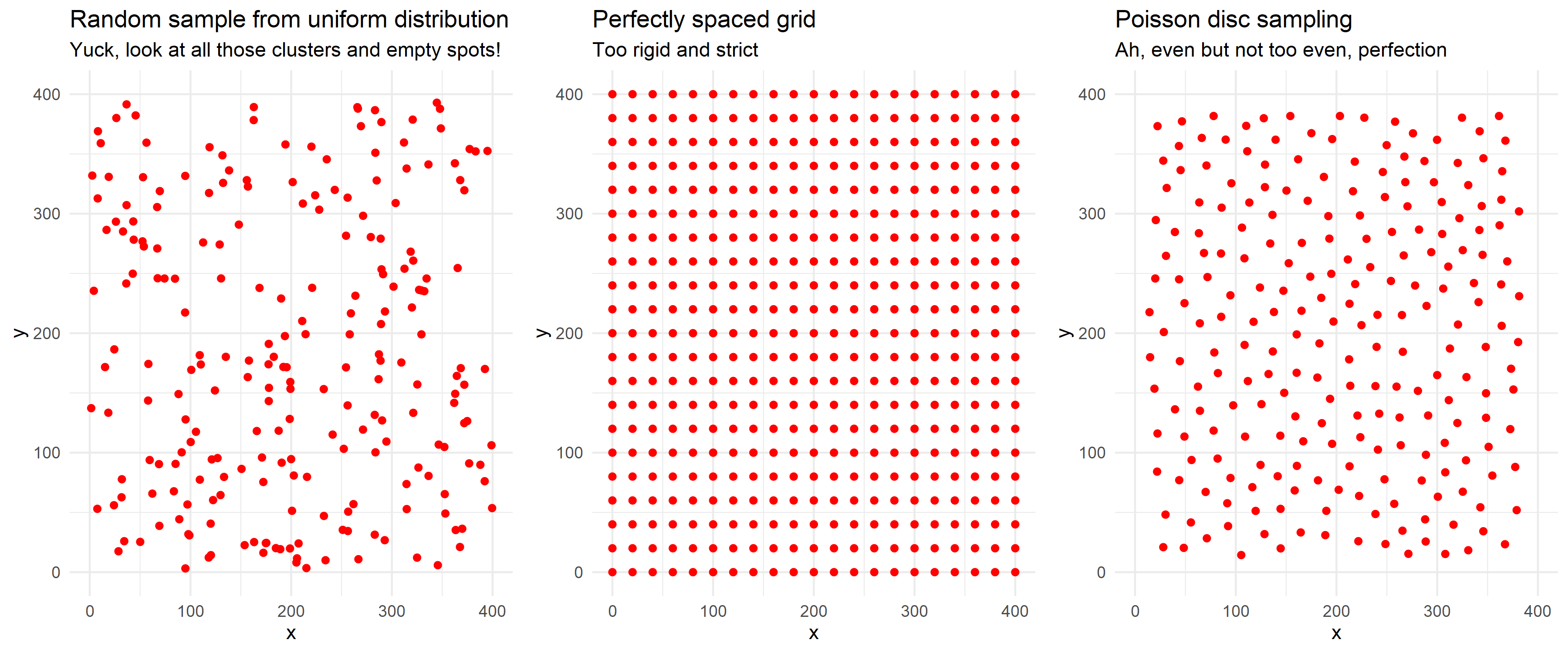
A few months back I wrote a package to implement Poisson Disc Sampling, which is an algorithm to generate points that are random but evenly spaced. Mine was basically just a port of a Javascript implementation, meaning it used lots of loops and was quite slow in R. Then @coolbutuseless came along and wrote his own version that was better in every possible way. My version is still around if you’re a glutton for punishment, but I myself have switched over to the far superior poissoned.

Drawing some shapes

To accompany the textures I was preparing, I planned some abstract geometric shapes as a canvas. There’s two main types: triangles and voronoi polygons. Both involve the same process, generate a set of seed points, calculate the voronoi tessellation or delaunay triangulation using the deldir package, and then filter out a portion of the shapes either by size or randomly. Here’s an example of generating a random set of triangles that are filtered by area.

library(tidyverse)
library(deldir)

#generate random seed points and calculate the delaunay triangulation
rand_pts <- data.frame(x = runif(50, 0, 300), y = runif(50, 0, 800))
tess <- deldir(rand_pts)
triang <- triang.list(tess)

triang_area <- function(data) {
  x <- data$x
  y <- data$y
  mat <- matrix(data = c(1,1,1,x[1],x[2],x[3],y[1],y[2],y[3]), nrow = 3, ncol = 3, byrow = TRUE)
  area <- 0.5*det(mat)
  return(area)
}

#add area to each triangle and do some reshuffling
triang %>%
  map( ~mutate(.x, area = triang_area(.x))) %>%
  bind_rows(.id = "id") %>%
  select(id, x, y, area) -> triang_df

#filter out smaller triangles
big_triang <-
  triang_df %>%
  group_by(id) %>%
  filter(area > 3000) %>%
  ungroup()

Adding texture

We can add some texture to our shapes by adding some very small and closely-spaced points generated by Poisson Disc Sampling. I’ll also use mgcv::in.out() to determine which points are inside or outside of the shapes we generated and color them differently.

library(poissoned)
library(mgcv)

#we'll use these later for texture
salt <- poisson_disc(300, 800, 1, k = 10, verbose = TRUE)
pepper <- poisson_disc(300, 800, 1, k = 10, verbose = TRUE)

#set up the boundary for each triangle
boundary <-
  split(big_triang, big_triang$id) %>%
  map( ~add_row(.x, id = NA, x = NA, y = NA, area = NA)) %>%
  bind_rows() %>%
  select(x, y)

#find the points inside and outside of the boundary
salt_inout <- in.out(as.matrix(boundary), as.matrix(salt))
salt_inside <- cbind(salt, salt_inout) %>%
  filter(salt_inout == TRUE)

pepper_inout <- in.out(as.matrix(boundary), as.matrix(pepper))
pepper_outside <- cbind(pepper, pepper_inout) %>%
  filter(pepper_inout == FALSE)

#color triangles
colors <- c("#E1BABA", "#FFDFE2", "#AAD8A8", "#8B9DC3", "#5C8492", "#B20937", "#E9FA77", "#D7EAAE", "#667788",
            "#761409", "#FFDD4D", "#aebab7", "#a3a3a3")
big_triang <-
  big_triang %>%
  group_by(id) %>%
  mutate(color = sample(colors, 1, replace = TRUE))

#plot
ggplot() +
  geom_polygon(data = big_triang, aes(x = x, y  = y, group = id, fill = color), color = "white", size = 1) +
  geom_point(data = salt_inside, aes(x = x, y = y), size = 0.001, color = "white", alpha = 0.15) +
  geom_point(data = pepper, aes(x = x, y = y), size = 0.1, color = "black", alpha = 1, shape = "*") +
  scale_fill_identity() +
  lims(x = c(0, 300), y = c(0, 800)) +
  theme_void()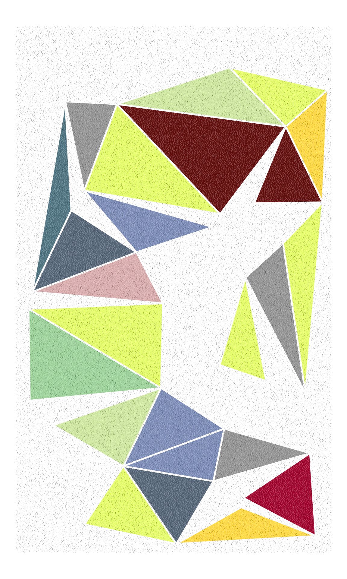

Animated color gradients

Our last example used a texture with lots of closely packed points. What if we made those points bigger, gave them some transparency, and colored them by point-of-discovery? Well then we’d have a very nice color gradient, and one that’s animatable to boot. There’s much more efficient ways to build color gradients in R, but this one has a couple of advantages: ordering by point of discovery isn’t a perfectly smooth gradient, there’s little blips and imperfections that give the final piece a nice organic feel, and since we’re using points and the poisson disc algorithm discovers points in a circle, we can make a nice animation.

library(tidyverse)
library(poissoned)
library(gganimate)

#generate a bunch of points around a center point with close distance and order of discovery kept
pts <- poisson_disc(ncols = 150, nrows = 400, cell_size = 2, xinit = 150, yinit = 750, keep_idx = TRUE) %>%
  arrange(idx)

#plot giving a color gradient based on order of discovery
ggplot(pts) +
  geom_point(aes(x = x, y = y, color = idx), size = 4, alpha = 0.9) +
  scale_color_gradientn(colors = c("#F37374", "#F48181", "#F58D8D","#FF9999", "#FFA3A3","#FFA699", "#FFB399", "#FFB399","#FFC099", "#FFC099","#FFCC99", "#FFCC99"), guide = "none") +
  theme_void()

#static image
#ggsave("sunrise.png", width = 5, height = 10)

#animate
anim <-
  ggplot(pts) +
  geom_point(aes(x = x, y = y, color = idx, group = idx), size = 4, alpha = 0.9) +
  scale_color_gradientn(colors = c("#F37374", "#F48181", "#F58D8D","#FF9999", "#FFA3A3","#FFA699", "#FFB399", "#FFB399","#FFC099", "#FFC099","#FFCC99", "#FFCC99"), guide = "none") +
  theme_void()  +
  scale_y_reverse() +
  transition_reveal(along = idx) +
  ease_aes("cubic-in") +
  enter_grow() +
  enter_fade(alpha = 0.9)

animate(anim, nframes = 100, fps = 20)
#anim_save("sunrise.gif")

Pebbles

Voronoi diagrams are fun, and I wanted to use them to make some generative pebbles. Taking inspiration from geom_shape() from the ggforce package, I wrote a function to take some voronoi polygons (or any polygon for that matter) and either expand or contract them using polyclip::polygon_offset(). To make some pebbles, all we need to do is pass a dataframe of polygons to shapify() setting the delta argument as some negative value to contract the polygons a little, and then going in for another pass with shapify() using a positive delta and miter = "round" to round the corners.

I also wrote some functions to generate a randomly sampled set of voronoi polygons, and to take a dataframe of polygons and a dataframe of points and select the points within the polygons. All of these functions are easily pipeable with the %>% operator from magrittr to make it easy to generate sets of pebbles with texture. Here’s an example that generates some pebbles with color gradients.

library(tidyverse)
library(rlang)
library(poissoned)
library(deldir)
library(rlist)
library(magrittr)
library(polyclip)
library(mgcv)


####################################
###Some general purpose functions###
####################################

#takes a dataframe of polygons (with id column) and dataframe of points (x, y)
#and returns a dataframe of points that are inside the polygons and classified
#by the id of the original polygon. Format (x, y, id)
texturize <- function(polys, pts) {
  polys %>%
    select(x, y) %>%
    split(., polys$id) %>%
    map(., ~in.out(as.matrix(.x), as.matrix(pts))) %>%
    map(., ~cbind(.x, pts)) %>%
    map(., ~rename(.x, "inout" = ".x")) %>%
    map(., ~filter(.x, inout == TRUE)) %>%
    bind_rows(.id = "id") %>%
    select(-inout)
}

#functions for reformatting deldir outputs
cleanup <- function(x) x[ !names(x) %in% c("pt", "ptNum", "area", "id")]
cleanup2 <- function(x) x[ !names(x) %in% c("x", "y", "ptNum", "area", "id", "bp")]

#generates a set of voronoi polygons filtered by area
#number of seed points is num_points
#canvas size is x_max and y_max
#max_size and min_size is the max and min area of the resulting voronoi polygons
#polygons outside of the min/max will be removed
medium_voronois <- function(num_points = 50, x_max = 300, y_max = 800, max_size = 8000, min_size = 3000) {
  rand_pts <- data.frame(x = runif(num_points, 0, x_max), y = runif(num_points, 0, y_max))
  tess <- deldir(rand_pts)
  vor_list <- tile.list(tess)

  vor_list_small <-
    vor_list %>%
    keep( ~ .x$area < max_size) %>%
    keep( ~ .x$area > min_size)

  vor_list_small %>%
    map( ~cleanup(.x)) %>%
    bind_rows(.id = "id") %>%
    select(id, x, y) %>%
    mutate(id = as.numeric(id))
}

#generates a set of voronoi polygons with specified num of seed pts and canvas size
#then randomly selects a certain number (num_shapes) to keep, and discards the rest
rand_voronois <- function(num_points = 50, x_max = 300, y_max = 800, num_shapes = 10) {
  rand_pts <- data.frame(x = runif(num_points, 0, x_max), y = runif(num_points, 0, y_max))
  tess <- deldir(rand_pts)
  vor_list <- tile.list(tess)

  vor_list_sample <- list.sample(vor_list, num_shapes)

  vor_list_sample %>%
    map( ~cleanup(.x)) %>%
    bind_rows(.id = "id") %>%
    select(id, x, y) %>%
    mutate(id = as.numeric(id))
}

#takes a dataframe of polygons and applies a shape manipulation
#polyclip::polyoffset has details on the parameters
shapify <- function(data, delta, jointype, miterlim = 2) {
  x_new <- split(data$x, data$id)
  y_new <- split(data$y, data$id)
  polygons <- Map(list, x = x_new, y = y_new)

  polygons2 <- lapply(polygons, polyoffset, delta = delta,
                      jointype = jointype, miterlim = miterlim)

  polygons2 %>%
    map(~as.data.frame(.x)) %>%
    bind_rows(.id = "id")
}

#list of color palettes
pals <- list(
  pal1 = colorRampPalette(colors = c("#daeed8", "#A4C990")),
  pal2 = colorRampPalette(colors = c("#FAEBD7", "#FF7373")),
  pal3 = colorRampPalette(colors = c("#B0E0E6", "#323232")),
  pal6 = colorRampPalette(colors = c("#efe1ff", "#bd3037"))
)

#takes an input dataframe of points with (x, y, id)
#and adds a color column that will make each set of points (each id group)
#a random gradient palette from the list of `pals`
colorize <- function(data) {
  dir <- sample(exprs(x, y, desc(x), desc(y)))[[1]]
  pal <- sample(pals)[[1]]

  data %>%
    arrange(!!dir) %>%
    mutate(color = pal(nrow(data)))
}

##############################################

##make some gradient colored pebbles
salt <- poisson_disc(ncols = 800, nrows = 2000, cell_size = 0.5, verbose = TRUE)
salt$x <- salt$x - 50
salt$y <- salt$y - 60

shapes <- medium_voronois(max_size = 11000) %>%
  shapify(delta = -30, jointype = "miter", miterlim = 1000) %>%
  shapify(delta = 20, jointype = "round") %>%
  texturize(salt)

tex_colored <-
  split(shapes, shapes$id) %>%
  map( ~colorize(.x)) %>%
  bind_rows()

ggplot() +
  geom_point(data = tex_colored, aes(x = x, y = y, color = color), alpha = 0.8, size = 2) +
  scale_color_identity() +
  theme_void() +
  theme(plot.background = element_rect(fill = "#EEE0E5"))

#ggsave("gradient_rocks.png", height = 11, width = 6)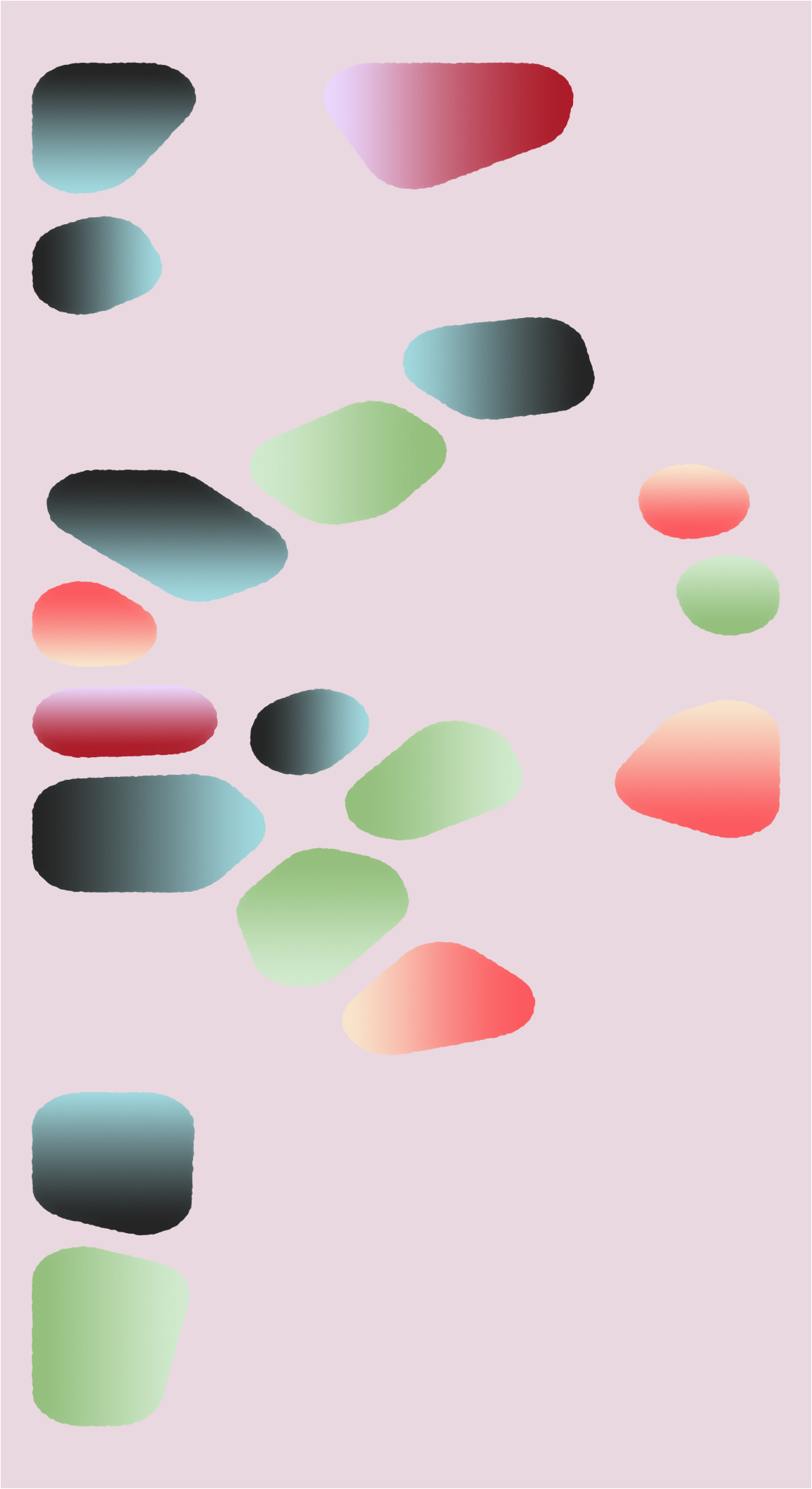

Circular pebble arrangement

I made a lot of these sketches with random voronoi layouts, and after a while I got tired of the randomness, and wanted a more directed layout. So I wrote a set of functions to place the voronoi pebbles in a set of concentric circles and then sample from those. Here’s a few more sketches I made. The first set is inspired by Alexander Calder’s Mobiles and the second set applies some randomized voronoi stippling that varies the size and color of the voronoi textures.

##NOTE: this continues from the above script, and relies on functions like shapify(), etc


#takes an input dataframe of seed points (x, y) and returns the voronoi tessellation as
#a dataframe with (x, y, id) ready for ggplotting
voronize <- function(data) {
  tess <- deldir(as.data.frame(data))
  vor_list <- tile.list(tess)

  vor_list %>%
    map( ~cleanup(.x)) %>%
    bind_rows(.id = "id") %>%
    select(id, x, y) %>%
    mutate(id = as.numeric(id))
}

#takes a set of points, and returns the points with their associated voronoi polygon IDs
#only reason this exists is to correlate polygon ID with seed point ID
get_seeds <- function(data) {
  tess <- deldir(as.data.frame(data))
  vor_list <- tile.list(tess)

  vor_list %>%
    map( ~as.data.frame(t(unlist(cleanup2(.x))))) %>%
    bind_rows(.id = "id") %>%
    select(id, pt.x, pt.y) %>%
    mutate(id = as.numeric(id))
}

#draws num_points in a circle, badly
#min_r and max_r are the min and max radius possible
#jitter is the x y randomness
bad_circle <- function(num_pts = 10, min_r, max_r, jitter) {
  tibble(angle = seq(0, 2*pi, length.out = num_pts), r = sample(seq(min_r, max_r, length.out = 100), num_pts, replace = TRUE)) %>%
    mutate(x_jitter = sample(seq(-jitter, jitter, length.out = 100), num_pts, replace = TRUE),
           y_jitter = sample(seq(-jitter, jitter, length.out = 100), num_pts, replace = TRUE),
           x = r*cos(angle) + x_jitter,
           y = r*sin(angle) + y_jitter) %>%
    select(x, y)
}

#draw concentric circles of pebbles then select some to keep
circle_pebbles <- function(num_pts = 10, min_r1 = 50, max_r1 = 100, jitter_1 = 100, min_r2 = 200, max_r2 = 300, jitter_2 = 100,
                           min_r3 = 400, max_r3 = 500, jitter_3 = 100, expand = -30, round = 20, num_keepers = 8, probs = NULL) {
  circle1 <- bad_circle(num_pts, min_r1, max_r1, jitter_1)
  circle2 <- bad_circle(num_pts, min_r2, max_r2, jitter_2)
  circle3 <- bad_circle(num_pts, min_r3, max_r3, jitter_3)

  all_circles <- rbind(circle1, circle2, circle3)

  circular_layer <- voronize(all_circles) %>%
    shapify(delta = expand, jointype = "miter", miterlim = 1000) %>%
    shapify(delta = round, jointype = "round")

  keepers <- sample(1:30, num_keepers, prob = probs)

  seeds <- get_seeds(all_circles) %>%
    filter(id %in% keepers)

  pebbles <-
    circular_layer %>%
    filter(id %in% keepers)

  list(seeds = seeds, pebbles = pebbles)
}

#make some Calder inspired diagrams
probs1 <- c(0.03, 0.03, 0.03, 0.03, 0.03, 0.03, 0.03, 0.03, 0.03, 0.03,1, 1, 1, 1, 1, 1, 1, 1, 1, 1, 0.03, 0.03, 0.03, 0.03, 0.03, 0.03, 0.03, 0.03, 0.03, 0.03)

circ_layer1 <- circle_pebbles(probs = probs1, num_keepers = 3)
circ_layer2 <- circle_pebbles(probs = probs1, num_keepers = 3)
circ_layer3 <- circle_pebbles(probs = probs1, num_keepers = 3)
circ_layer4 <- circle_pebbles(probs = probs1, num_keepers = 2)
circ_layer5 <- circle_pebbles(probs = probs1, num_keepers = 2)

ggplot() +
  geom_segment(data = circ_layer1[["seeds"]], aes(x = pt.x, y = pt.y, xend = 0, yend = 0), color = "black", linetype = "dotted", alpha = 0.8) +
  geom_segment(data = circ_layer2[["seeds"]], aes(x = pt.x, y = pt.y, xend = 0, yend = 0), color = "black", linetype = "dotted", alpha = 0.8) +
  geom_segment(data = circ_layer3[["seeds"]], aes(x = pt.x, y = pt.y, xend = 0, yend = 0), color = "black", linetype = "dotted", alpha = 0.8) +
  geom_segment(data = circ_layer4[["seeds"]], aes(x = pt.x, y = pt.y, xend = 0, yend = 0), color = "black", linetype = "dotted", alpha = 0.8) +
  geom_segment(data = circ_layer5[["seeds"]], aes(x = pt.x, y = pt.y, xend = 0, yend = 0), color = "black", linetype = "dotted", alpha = 0.8) +
  geom_polygon(data = circ_layer1[["pebbles"]], aes(x = x, y = y, group = id), fill = "#10628E", alpha = 0.85) +
  geom_polygon(data = circ_layer2[["pebbles"]], aes(x = x, y = y, group = id), fill = "#D42A20", alpha = 0.85) +
  geom_polygon(data = circ_layer3[["pebbles"]], aes(x = x, y = y, group = id), fill = "#FAC12C", alpha = 0.85) +
  geom_polygon(data = circ_layer4[["pebbles"]], aes(x = x, y = y, group = id), fill = "black", alpha = 0.85) +
  geom_polygon(data = circ_layer5[["pebbles"]], aes(x = x, y = y, group = id), fill = "white", alpha = 0.85) +
  theme_void() +
  theme(plot.background = element_rect(fill = "#FCF3D9"))

#ggsave("calder_pebbles.png", height = 8, width = 8)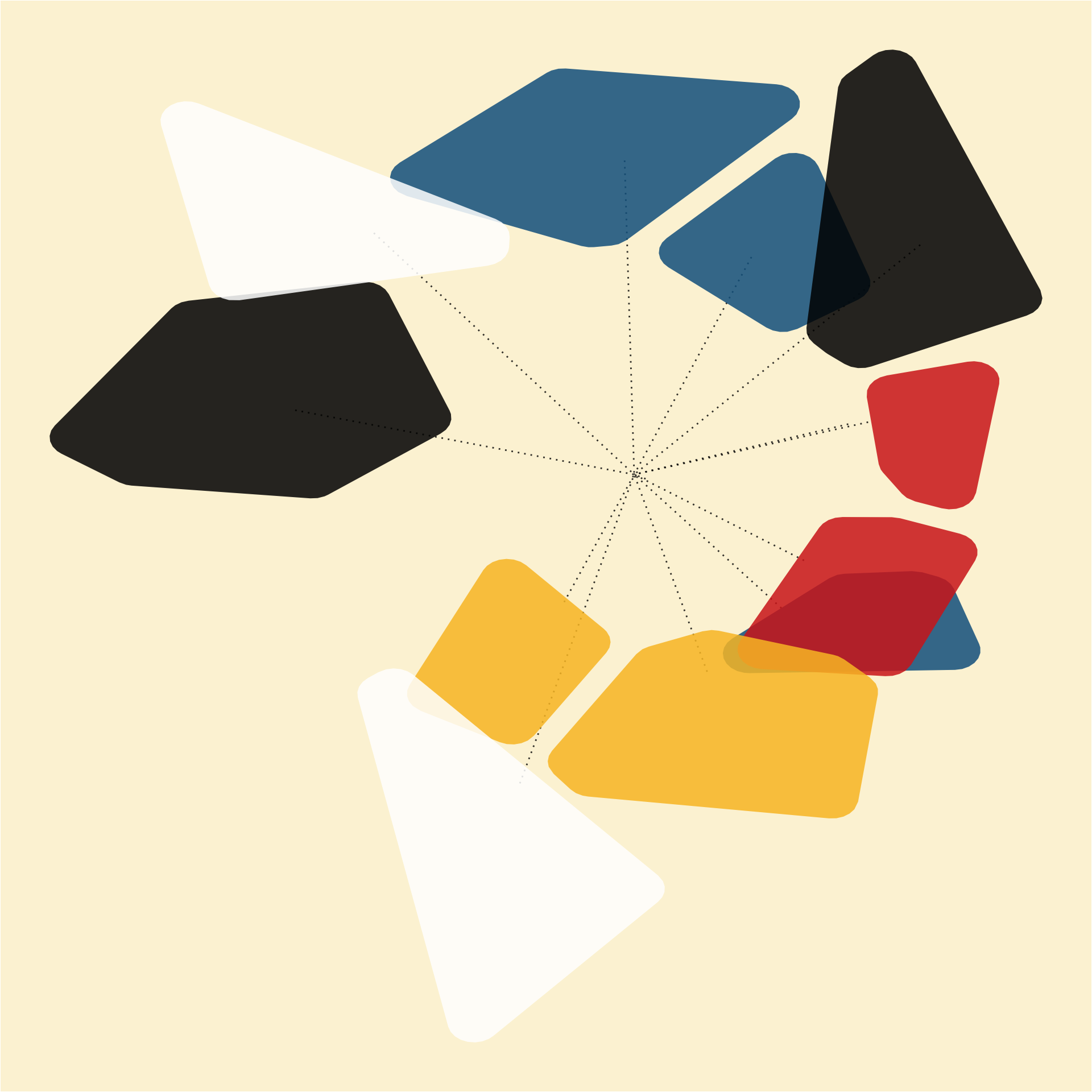

#make some textured pebbles
probs2 <- c(0.05, 0.05, 0.05, 0.05, 0.05, 0.05, 0.05, 0.05, 0.05, 0.05,1, 1, 1, 1, 1, 1, 1, 1, 1, 1, 0.05, 0.05, 0.05, 0.05, 0.05, 0.05, 0.05, 0.05, 0.05, 0.05)
pebble_colors <- c('#20342a', '#f74713', '#686d2c', '#e9b4a6')
tex_colors <- c('#4d3d9a', '#f76975', '#ffffff', '#eff0dd')
pts <- poisson_disc(ncols = 400, nrows = 400, cell_size = 5.5, k = 10, verbose = TRUE)
pts$x <- pts$x - 1000
pts$y <- pts$y - 1000

circ_layer6 <- circle_pebbles(probs = probs2, num_keepers = 20)[["pebbles"]] %>%
  group_by(id) %>%
  group_map( ~mutate(.x, color = sample(pebble_colors, 1))) %>%
  ungroup()

tex_colored <-
  texturize(circ_layer6, pts)  %>%
  mutate(size = sample(seq(0.03, 0.6, length.out = 100), size = nrow(.), replace = TRUE)) %>%
  group_by(id) %>%
  group_map( ~mutate(.x, color = sample(tex_colors, 1))) %>%
  ungroup()

tex_random <-
  tex_colored %>%
  sample_n(nrow(tex_colored) / 10) %>%
  mutate(color = sample(tex_colors, nrow(.), replace = TRUE))

tex_final <- left_join(tex_colored, tex_random, by = c("x", "y")) %>%
  mutate(color.x = ifelse(is.na(color.y), color.x, color.y)) %>%
  select(id = id.x, x, y, size = size.x, color = color.x)

ggplot() +
  geom_polygon(data = circ_layer6, aes(x = x, y = y, group = id, fill = color)) +
  geom_point(data = tex_final, aes(x = x, y = y, size = size, color = color)) +
  scale_fill_identity() +
  scale_color_identity() +
  scale_size_identity() +
  theme_void() +
  theme(plot.background = element_rect(fill = "#e5ded8"))

#ggsave("textured_pebbles.png", height = 10, width = 10)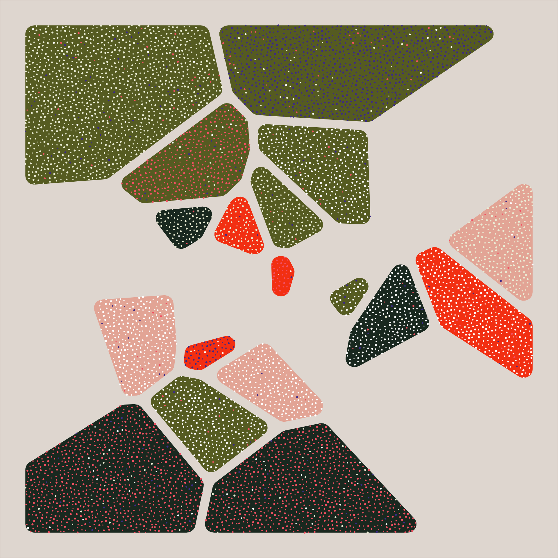

Endless possibilites

This post has just scratched the surface of what’s possible. I love working with abstract sketches like this because it’s a great way to study color, layout, shapes, and all sorts of other important concepts. I hope you can take these ideas and extend them for your own studies. Consider combining shapes, overlaying shapes, creating new textures by using unicode glyphs, or whatever else you can come up with! As always, all of the code is on my GitHub. Have fun!