Noise (12 Months of aRt, August)

August 30, 2019

Turn up the noise

Very few algorithms are award-winning, and even fewer have won an Academy Award. Today’s topic however, can claim this rare honor. In 1982, Ken Perlin developed the Perlin Noise algorithm to generate random procedural textures for Disney’s sci-fi classic Tron. In 1997, Ken won the Academy Award for technical achievement, in large part thanks to his eponymous noise algorithm. In this post, I’ll explore several types of noise, and the modifications we can apply to them. This is all centered around the Ambient package, by Thomas Lin Pedersen (I mean, who else would it be?).

I won’t pretend that I understand the math behind noise algorithms, but I’ll at least try to describe what some of our options are and how they can influence the output. Let’s meet the players: noise generating algorithms include Perlin, OpenSimplex, Worley, Cubic, and more, and some of these include parameters than can be tweaked to change the values and appearance of the generated noise. Let’s demonstrate using one-dimensional Perlin noise.

library(dplyr)
library(ggplot2)
library(ambient)

#we can use ambient::long_grid to help us generate a tidy data structure for calculating noise
grid <- long_grid(1, seq(1, 10, length.out = 1000))

#now calculate perlin noise for the grid
grid$noise <- gen_perlin(x = grid$x, y = grid$y)

#extract our noise as a 1D line
line <- data.frame(x = seq(1:1000), y = grid$noise[1:1000])

ggplot(line) +
  geom_line(aes(x = x, y = y), size = 1)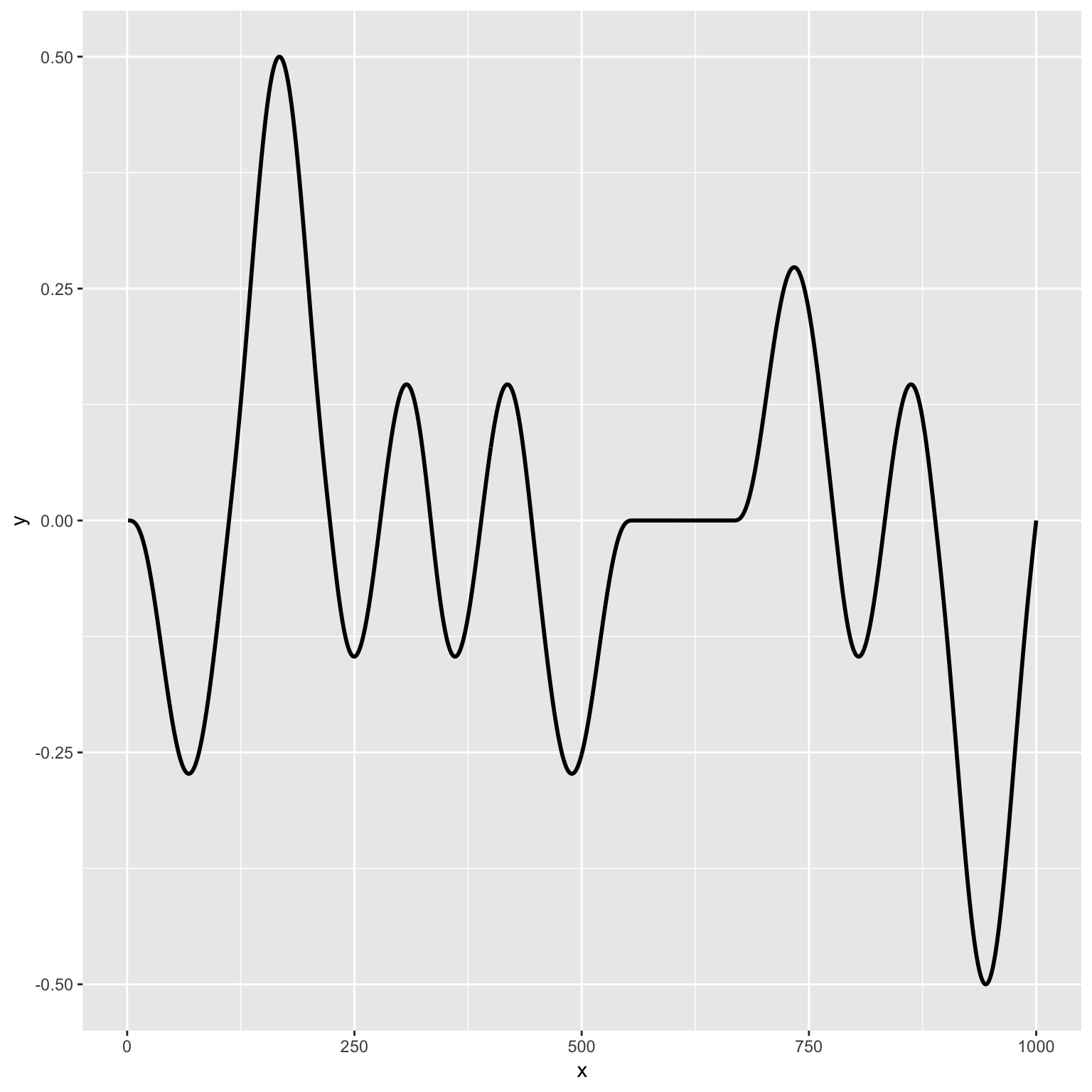

We can see that this produces a sort of wavy up and down pattern. If we want more randomness we can apply a fractal to the noise, which is more in line with how Perlin noise is typically calculated. There are several types of fractals, which can all be applied with ambient::fracture. You can read about the options on the Ambient website, but here I will just use fbm which is the most common type.

grid <- long_grid(1, seq(1, 10, length.out = 1000))
grid$noise <- fracture(gen_perlin, fbm, octaves = 5, x = grid$x, y = grid$y)

line <- data.frame(x = seq(1:1000), y = grid$noise[1:1000])

ggplot(line) +
  geom_line(aes(x = x, y = y), size = 1)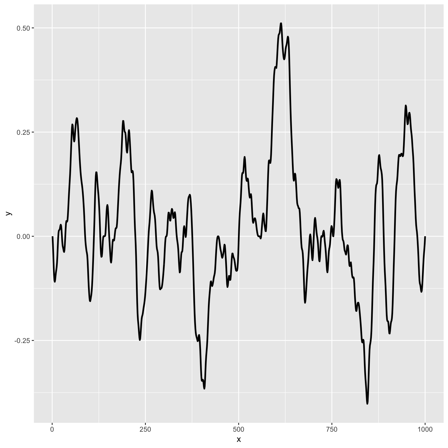

Now our line appears much more spiky and fractured (go figure!). But hold on, if you’ve ever seen Perlin noise, you’re probably thinking it doesn’t look anything like these graphs above. That’s because typically noise is presented in two or three or even four dimensions. Well, let’s take a bunch of those 1D vectors, line them up into a grid, and now we’ve got an intensity matrix—cool! Next let’s move on to more noise, more fractals, and more weirdness (all in 2D from here on).

Worley noise

Worley noise is a type of point-based noise that bares some resemblance to Voronoi diagrams. You can see typical examples on the Ambient website, but I’m not here to just recreate the defaults, so let’s explore some of the parameters. Changing the value parameter to "distance2sub" will give us a diagram that resembles crystals or gemstones.

grid <-
  long_grid(seq(1, 10, length.out = 1000), seq(1, 10, length.out = 1000)) %>%
  mutate(noise = gen_worley(x, y, value = "distance2sub"))

ggplot() +
  geom_raster(data = grid, aes(x, y, fill = noise)) +
  theme_void() +
  theme(legend.position = "none")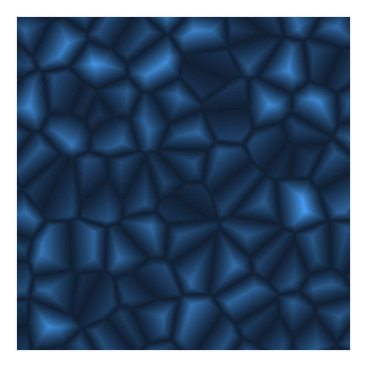

We can also mess with the jitter and distance_ind parameters, which to my eye, has the effect of making the diagram more ‘gridded’ or random. Here I’m upping the distance index and lowering the jitter slightly from the default.

grid <-
  long_grid(seq(1, 10, length.out = 1000), seq(1, 10, length.out = 1000)) %>%
  mutate(noise = gen_worley(x, y, value = "distance2sub", jitter = 0.4, distance_ind = c(1, 5)))

ggplot() +
  geom_raster(data = grid, aes(x, y, fill = noise)) +
  scale_fill_gradientn(colors = c("black", "#47C2C9", "#E384BD", "white")) +
  theme_void() +
  theme(legend.position = "none")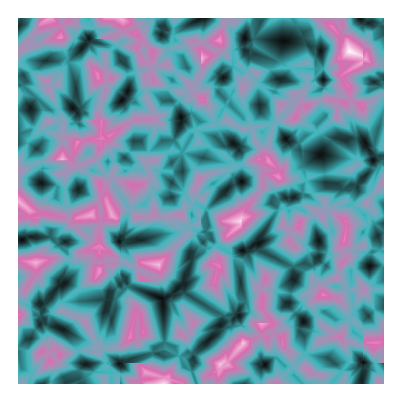

Fractals

As discussed above, we can apply a fractal to these noise algorithms to introduce more frequent variations. Ambient comes with several types of fractals, including the standard fractal brownian motion fbm, but also billow, ridged, clamped, and spectral_gain. Within each of these fractals you can set the octaves which will increase the number of generated values to combine, essentially higher octaves will have more frequent fractures or more randomness. I particularly love the ridged fractal, so let’s see how we can use it with Worley noise.

grid <-
  long_grid(x = seq(1, 10, length.out = 1000), y = seq(1, 10, length.out = 1000)) %>%
  mutate(fractal = fracture(gen_worley, ridged, value = "distance2div", octaves = 8, x = x, y = y))

ggplot() +
  geom_raster(data = grid, aes(x, y, fill = fractal)) +
  theme_void() +
  theme(legend.position = "none")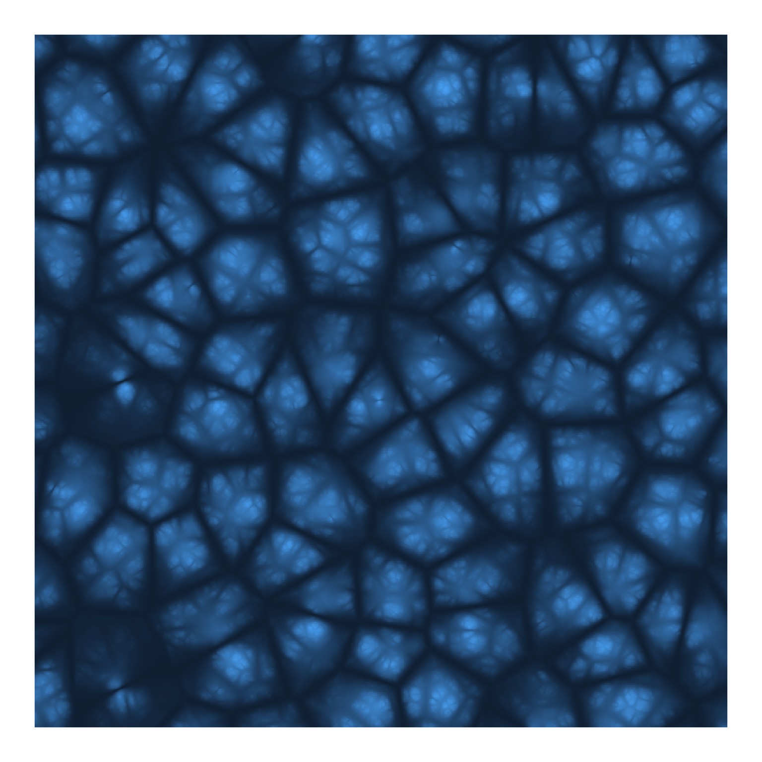

I love this one, the fractal creates something that resembles depth-of-field, and it reminds me of some sort of alien pod out of a sci-fi movie.

Perturbation

I often bother Thomas on Twiter with my #lazyweb questions, and he’s always very kind and gives me helpful answers like this one where I asked how I could achieve perturbation with the Ambient tidy interface:

He told me perturbation is really just adding noise to the coordinates before calculating your noise function. This really got me thinking, and led me down the path of augmenting the x and y seed coordinates with various levels of noise, then calculating noise from these warped coordinates.

grid <-
  long_grid(x = seq(0, 10, length.out = 1000),
            y = seq(0, 10, length.out = 1000)) %>%
  mutate(
    x1 = x + gen_perlin(x = x, y = y, frequency = 1),
    y1 = y + gen_perlin(x = x, y = y, frequency = 2),
    x2 = x1 + gen_simplex(x = x1, y = y1, frequency = 1),
    y2 = y1 + gen_simplex(x = x1, y = y1, frequency = 3),
    simplex_warp = gen_simplex(x = x1, y = y2)
  )

ggplot() +
  geom_raster(data = grid, aes(x, y, fill = simplex_warp)) +
  scale_fill_gradientn(colors = c('#253852', '#51222f', '#b53435', '#ecbb51', "#eeccc2"), guide = "none") +
  theme_void() +
  theme(legend.position = "none")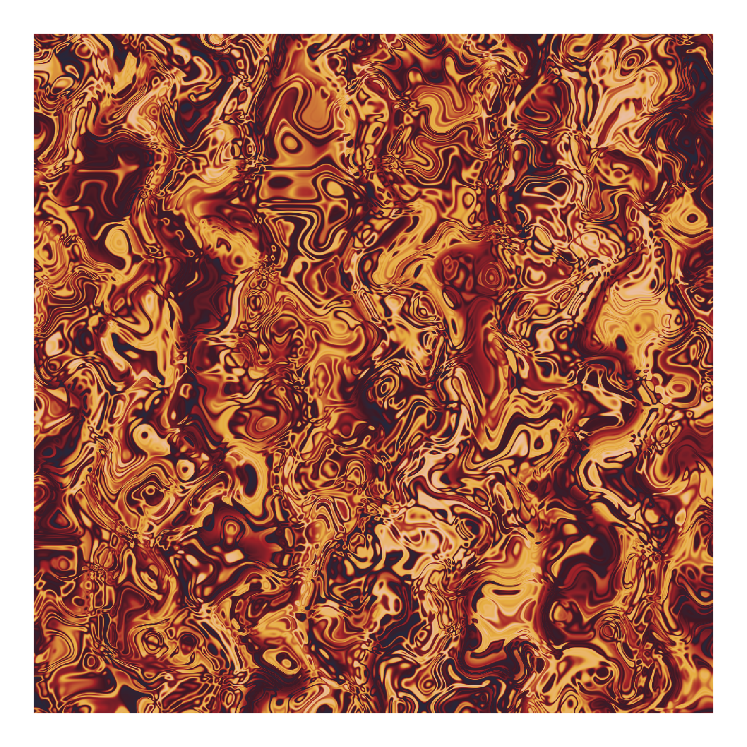

Putting it all together

Ambient contains a handy function blend that we can use to combine everything we’ve done so far. blend will take an input matrix and use it as a mask to blend two other matrices. Here’s a couple of my favorite examples using blend along with perturbation, fractals, and all the other goodness we’ve learned up to this point.

grid <-
  long_grid(x = seq(0, 10, length.out = 1000),
          y = seq(0, 10, length.out = 1000)) %>%
  mutate(
    x1 = x + gen_simplex(x, y) / 2,
    y1 = y + gen_simplex(x, y) * 2,
    worley = gen_worley(x, y, value = 'distance2mul', jitter = 0.5),
    simplex_frac = fracture(gen_simplex, ridged, octaves = 10, x = x, y = y),
    full = blend(normalise(worley), normalise(simplex_frac), gen_spheres(x1, y1))
  )

ggplot() +
  geom_raster(data = grid, aes(x, y, fill = full)) +
  scale_fill_gradientn(colors = c("black", "#DC1F24", "#EDE8E8","#4BC4CB"), guide = "none") +
  theme_void() +
  theme(legend.position = "none", plot.background = element_blank(), panel.background = element_blank())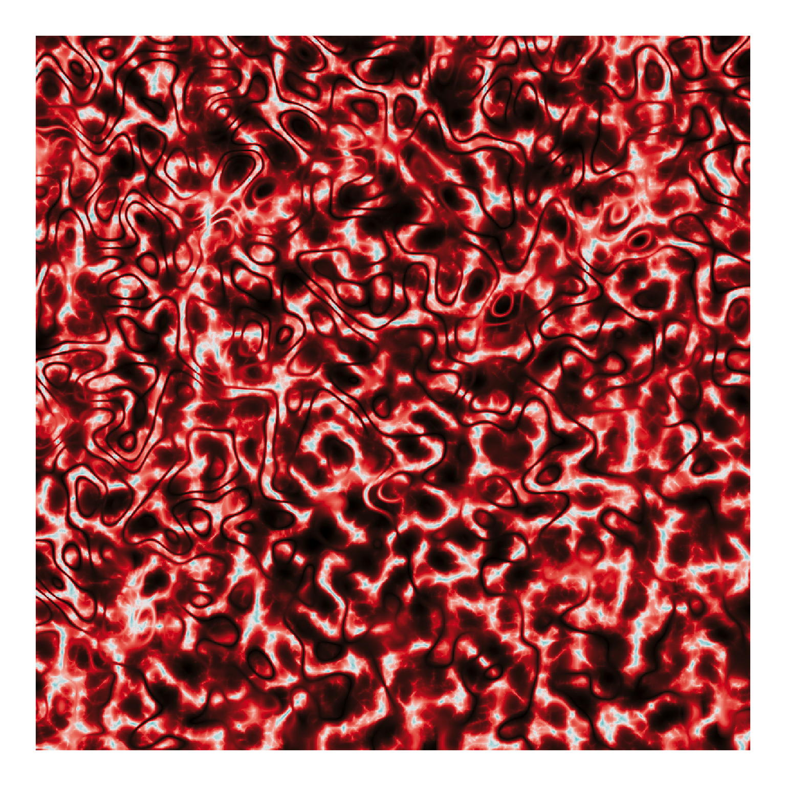

grid <- long_grid(seq(1, 10, length.out = 1000), seq(1, 10, length.out = 1000)) %>%
  mutate(
         x1 = x + fracture(gen_worley, ridged, octaves = 8, x = x, y = y, value = "distance2div", distance = "euclidean",
                           distance_ind = c(1, 2), jitter = 0.4),
         y1 = y + fracture(gen_worley, ridged, octaves = 8, x = x, y = y, value = "distance2div", distance = "euclidean",
                           distance_ind = c(1, 2), jitter = 0.4),
         simplex_warp = gen_worley(x = x1, y = y1, value = "distance")
         )

ggplot() +
  geom_raster(data = grid, aes(x, y, fill = simplex_warp)) +
  theme_void() +
  theme(legend.position = "none")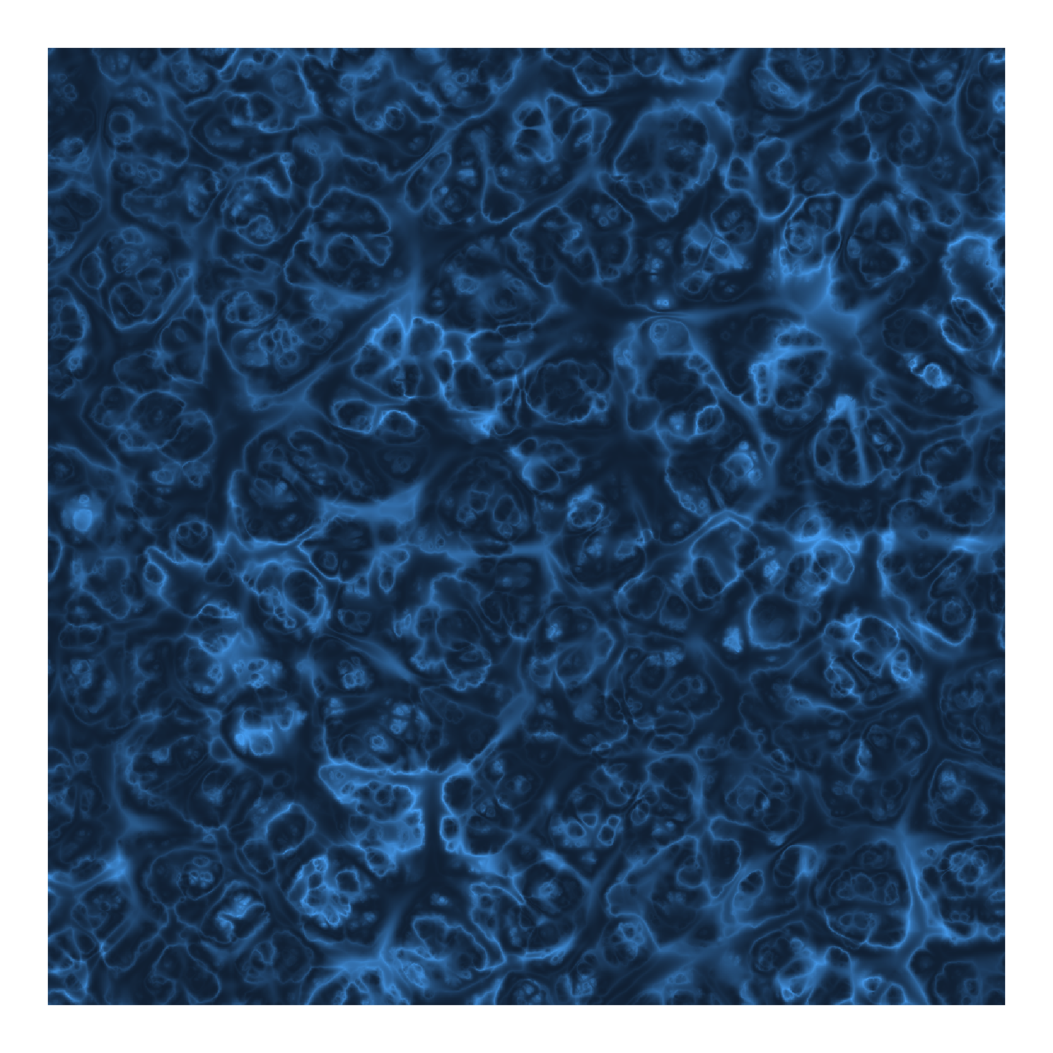

grid <- long_grid(seq(1, 10, length.out = 1000), seq(1, 10, length.out = 1000)) %>%
  mutate(
    x1 = x + fracture(gen_worley, ridged, octaves = 8, x = x, y = y, value = "distance2div", distance = "euclidean",
                      distance_ind = c(1, 2), jitter = 0.5),
    y1 = y + fracture(gen_worley, ridged, octaves = 8, x = x, y = y, value = "distance2div", distance = "euclidean",
                      distance_ind = c(1, 3), jitter = 0.4),
    worley_warp = gen_worley(x = x1, y = y1, value = "distance", jitter = 0.4, distance = "manhattan"),
    worley_warp2 = fracture(gen_worley, ridged, octaves = 8, x = x1, y = y1, value = "distance2div", distance = "euclidean",
                            distance_ind = c(1, 2), jitter = 0.5),
    cubic = gen_cubic(x = x * 3, y = y / 3),
    blend = blend(normalize(cubic), worley_warp, worley_warp2)
  )

ggplot() +
  geom_raster(data = grid, aes(x, y, fill = blend)) +
  scale_fill_gradientn(colors = c('#f0efe2', '#363d4a', '#7b8a56', '#ff9369', '#f4c172'), guide = "none") +
  theme_void() +
  theme(legend.position = "none")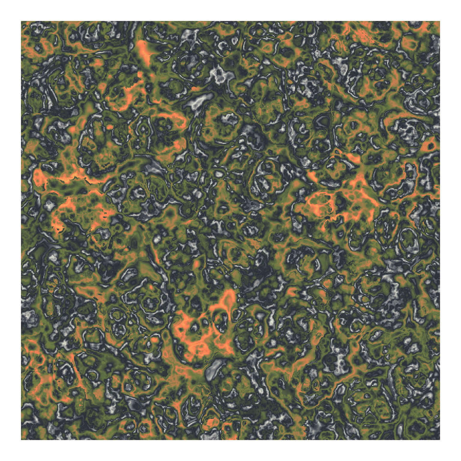

Wrapping up

You can see from these last couple examples that the possibilities are truly endless. I don’t want to calculate the actual number, but I’m pretty sure between noise parameters, fractals, perturbation, and blending there’s about 546,000,000,000,000 noise fields you could make with Ambient. Hopefully this post has given you a good idea of what’s possible, and the resources to get started. Be sure to check out the Ambient website, which has excellent documentation, and as always, you can get all the code for this post on my GitHub.