Flow fields (12 Months of aRt, September)

September 30, 2019

Flow fields are something we’ve circled for a while now. Back in February I wrote about strange attractors, which are a sort of flow field, and last month we explored noise functions, which is the perfect groundwork for today’s topic. A flow field is simply a grid of vectors, which is to say, it’s a grid of numbers. Flow fields can be generated by attractor functions, images, magnetic fields, wind, or what we will focus on today, noise functions.

Particles

You can visualize flow fields using arrows, glyphs, or as we will do now, particles. Thomas Lin Pedersen’s particles package will provide a useful interface for us to release some particles and let them flow through our field recording their position. We will then track the path of the particles which reveals the structure of our flow field. To make a particles picture out of a flow field, we’ll set up some particles and then run a simulation with a low velocity on the particles and allow the system to evolve over 50 or 100 generations**. We will steer the particles according to our flow field values, which can be converted from noise values to angles by normalizing to (-1, 1) and multiplying by 2π. I recommend reading of the particles vignette which is very helpful in understanding how to set up a simulation.

library(tidyverse)
library(ambient)
library(particles)
library(tidygraph)

#create noise field
grid <- long_grid(seq(1, 10, length.out = 1000), seq(1, 10, length.out = 1000)) %>%
  mutate(noise = gen_simplex(x, y))

#convert noise values to a matrix of angles
field <- as.matrix(grid, x, value = normalize(noise, to = c(-1, 1))) * (2 * pi)

#particle simulation, taken from {particles} vignette
sim <- create_ring(1000) %>%
  simulate(alpha_decay = 0, setup = aquarium_genesis()) %>%
  wield(reset_force, xvel = 0, yvel = 0) %>%
  wield(field_force, angle = field, vel = 0.1, xlim = c(-5, 5), ylim = c(-5, 5)) %>%
  evolve(100, record)

traces <- data.frame(do.call(rbind, lapply(sim$history, position)))
names(traces) <- c('x', 'y')
traces$particle <- rep(1:1000, 100)

#plot particle traces
ggplot(traces) +
  geom_path(aes(x, y, group = particle), size = 0.1) +
  theme_void() +
  theme(legend.position = 'none')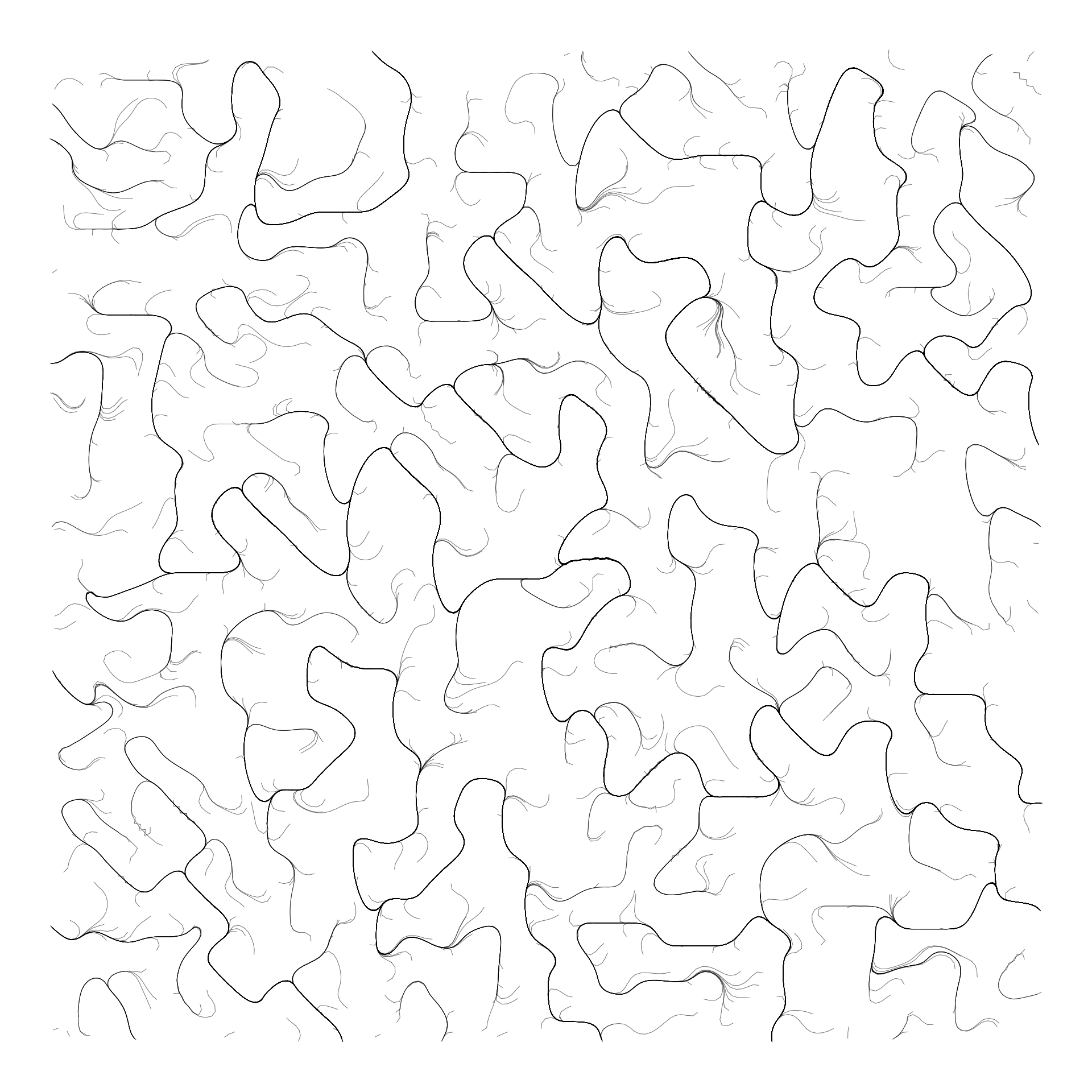

Curl noise

This isn’t necessarily wrong, but it’s not quite the look I want. Normal noise functions produce flow fields with lots of sinks, meaning that after a few generations of the simulation, all of the particles will converge on some valleys and remain there. This is why you see a bunch of dark lines with only a couple smaller lines coming out in this render. If we want a field that looks more fluid, we can use curl noise to produce a divergence-free flow field. Fields with sinks and gutters are said to have divergence but by applying curl noise to any continuous field like perlin or simplex noise, we can transform it to a form more suitable for our purposes.

grid <- long_grid(seq(1, 10, length.out = 1000), seq(1, 10, length.out = 1000)) %>%
  mutate(noise = gen_simplex(x, y))

curl <- curl_noise(gen_perlin, x = grid$x, y = grid$y)

grid$angle <- atan2(curl$y, curl$x) - atan2(grid$y, grid$x)

field <- as.matrix(grid, x, value = angle)

sim <- create_empty(1000) %>%
  simulate(alpha_decay = 0, setup = aquarium_genesis(vel_max = 0)) %>%
  wield(reset_force, xvel = 0, yvel = 0) %>%
  wield(field_force, angle = field, vel = 0.1, xlim = c(-5, 5), ylim = c(-5, 5)) %>%
  evolve(100, record)

traces <- data.frame(do.call(rbind, lapply(sim$history, position)))
names(traces) <- c('x', 'y')
traces$particle <- rep(1:1000, 100)

ggplot(traces) +
  geom_path(aes(x, y, group = particle), size = 0.3, alpha = 0.5) +
  theme_void() +
  theme(legend.position = 'none')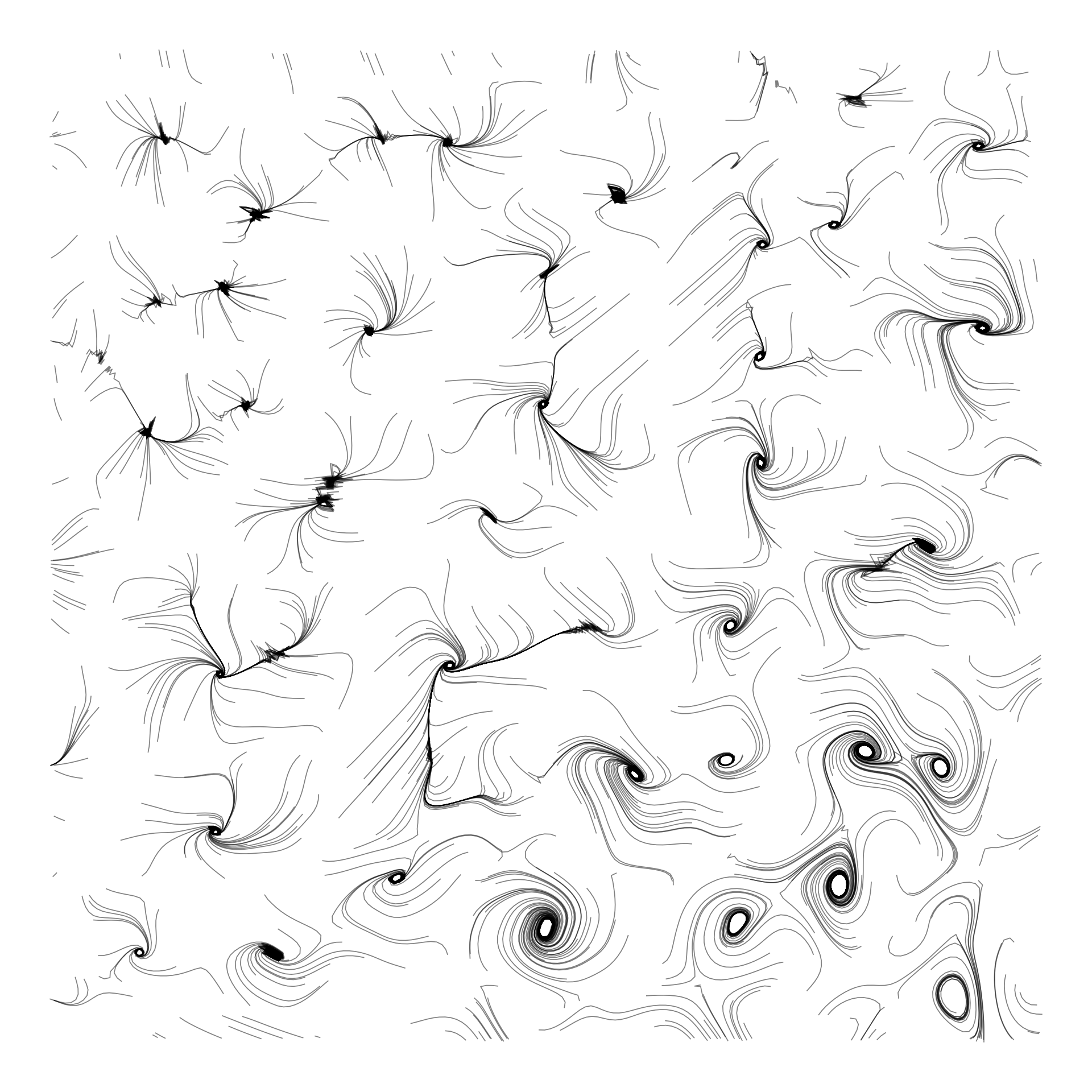

That looks much more fluid, now let’s examine how we handle curl noise. The curl_noise() function from ambient gives a transformed x and y for our original grid. When I first tested this, I didn’t realize you could actually feed these new coordinates directly to wield(), so instead I calculated the angle between the original point and the new point using some trigonometry. When I went back and tested it by directly plugging in the coordinates, I didn’t get the same type of fluid field result. I can’t nail down what exactly I’m doing wrong, but since my trig solution seems to produce something nice looking, I’m sticking with it (though be warned, it’s very possible I made a mistake here too and this is all just a happy accident r emo::ji("wink")).

From here the choice is yours. Use different noise parameters, try different particle layouts or velocities, different numbers of generations, grid sizes, colors, and anything else you can think of. One parameter I had fun playing with is xlim and ylim in wield(). These set the coordinate span in the x or y direction of our vector field. I’m sure you should set these to the actual span of your noise grid, but I just started setting them to random values and stumbled upon some lovely mistakes. I found that the sweet spot for a 1000x1000 grid is between 10 and 100. Here’s an example of messing with these parameters and adding color.

seed <- sample(1:2000, 1)

grid <-
  long_grid(x = seq(0, 10, length.out = 1000),
            y = seq(0, 10, length.out = 1000)) %>%
  mutate(
    x1 = x + gen_perlin(x = x, y = y, frequency = 2, seed = seed),
    y1 = y + gen_perlin(x = x, y = y, frequency = 0.5, seed = seed)
  )

curl <- curl_noise(gen_perlin, seed = seed, x = grid$x1, y = grid$y1)

grid$angle <- atan2(curl$y, curl$x) - atan2(grid$y, grid$x)

field <- as.matrix(grid, x, value = angle)

sim <- create_ring(10000) %>%
  simulate(alpha_decay = 0, setup = petridish_genesis(vel_max = 0, max_radius = 1)) %>%
  wield(reset_force, xvel = 0, yvel = 0) %>%
  wield(field_force, angle = field, vel = 0.15, xlim = c(-50, 40), ylim = c(-50, 40)) %>%
  evolve(100, record)

traces <- data.frame(do.call(rbind, lapply(sim$history, position)))
names(traces) <- c('x', 'y')
traces$particle <- rep(1:10000, 100)

bl_yl <- c('#4CA66B', '#00b2dd')
bl_yl_bg <- '#EEEEEE'

traces2 <-
  traces %>%
  group_by(particle) %>%
  mutate(color = sample(bl_yl, 1, replace = TRUE))

ggplot(traces2) +
  geom_path(aes(x, y, group = particle, color = color), size = 0.035, alpha = 0.6) +
  scale_color_identity(guide = "none") +
  theme_void() +
  theme(legend.position = 'none', panel.background = element_rect(fill = bl_yl_bg))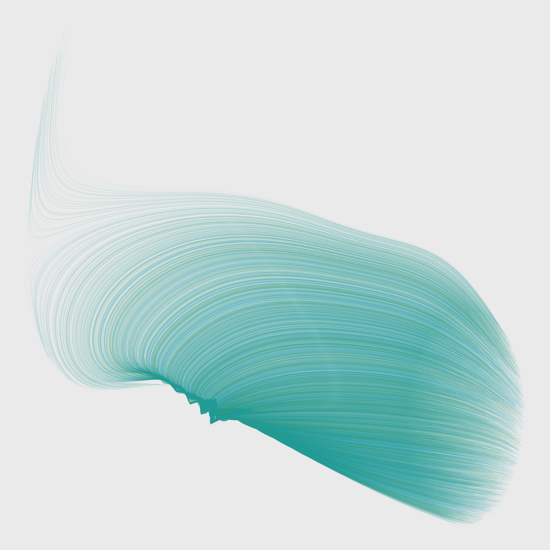

Polygons

Particles are just one of many ways to visualize flow fields. Here I’ll demonstrate another using polygons. This time we’ve got our original noise grid, then we can calculate angles directly from the noise grid, or compute the angles of the curl of the noise. We will map noise to some parameters like size and/or color, and map the polygon angle to the angle we’ve calculated for our grid. This makes use of geom_regon() from the ggforce package to render polygons of n sides at each point in our grid.

library(ggforce)

seed <- 111

grid <- long_grid(seq(1, 10, length.out = 50), seq(1, 10, length.out = 50)) %>%
  mutate(noise = gen_perlin(x, y, seed = seed))

curl <- curl_noise(gen_perlin, seed = seed, x = grid$x, y = grid$y)

grid$angle <- atan2(curl$y, curl$x) - atan2(grid$y, grid$x)

ggplot(grid) +
  geom_regon(aes(x0 = x, y0 = y, r = noise/3, angle = angle, sides = 3, fill = noise), alpha = 0.75) +
  scale_fill_gradientn(colors = c("#FFC1C1", "#C6B6E0", "#C6B6E0", "#326983"), guide = "none") +
  theme_void()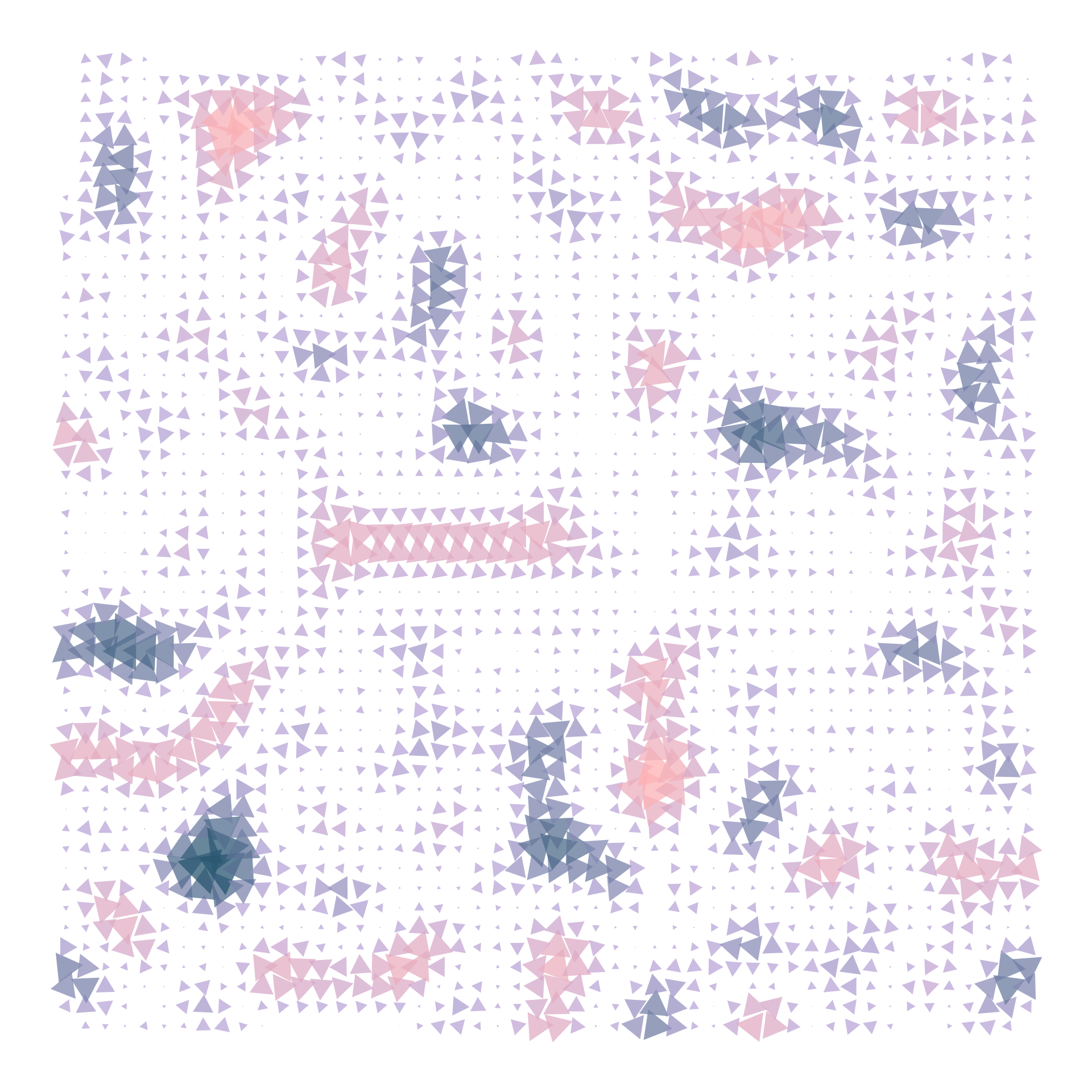

Just like with particles, we can change all sorts of parameters, like color, transparency, types of polygons, types of noise, etc. Here let’s try a fun variation with worley noise.

seed <- sample(1:1000, 1)

grid <-
  long_grid(x = seq(0, 10, length.out = 60),
            y = seq(0, 10, length.out = 60)) %>%
  mutate(noise = gen_worley(x, y, seed = seed))

curl <- curl_noise(gen_worley, seed = seed, x = grid$x, y = grid$y)

grid$angle <- atan2(curl$y, curl$x) - atan2(grid$y, grid$x)

ggplot(grid) +
  geom_regon(aes(x0 = x, y0 = y, r = noise/4, sides = 4, fill = noise, angle = angle), alpha = 0.8) +
  scale_fill_gradientn(colors = c("#009A72", "#2AA57E", "#6DB089", "#B9BA94", "#FFC4A0", "#FFAA94", "#FFA198", "#FFA9A8", "#FAC4C6"), guide = "none") +
  theme_void()

More pretty pictures

I hope you’ve enjoyed this post, and maybe learned something? If nothing else, perhaps you’ve seen that sometimes, it’s OK to not really understand what’s going on with generative art. A lot of these experiments were things I stumbled upon by accident or in pursuit of something else. Take what comes your way, and remember it’s about the art, not the code. Speaking of the code, you can find it, along with more pictures on my GitHub.

Here’s a selection of some of my favorite particle fields I made while exploring this month.