Disintegration, part 2 (12 Months of aRt, November)

February 16, 2020

Background

Welcome back! Last month, we developed a rather rudimentary particle system; this month, we’re going to give it a glow up. To remind you, our particle system of last time went something like this: make some shapes out of points, apply a force to the points in some direction, some of the particles move like they’re being carried away in the wind, while others stay put. It was nice, I liked the results, but we can always do more.

Improving our particle system

One of the issues with the previous system was that the moving particles were chosen randomly. That can be nice, but I want more control. I also found the parameters for describing the way that the particles moved were too simplistic, I wanted some more randomness and more dials to tweak. We were also limited to equally sized points in our previous system; today we’ll improve on that. And last but not least, we’ll work on everyone’s favorite: color.

More precision

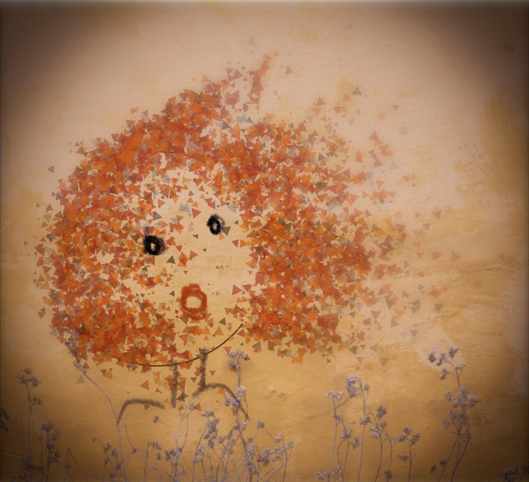
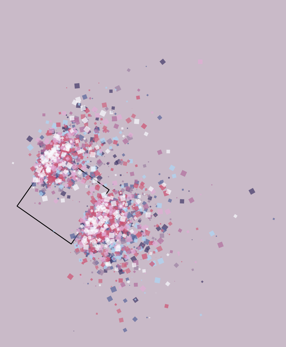
The randomness of our original algorithm was fun, but to give more control over the output, I added the ability to specify which particles should move and which should remain static. This is done by supplying the gaps parameter in the splitter() function with a list of vectors specifying the intervals of particles that should move. For example, by setting gaps = list(c(100, 500), c(1000, 2000)) particles 100 through 500, and 1000 through 2000 will move, while the rest will stay put. If you leave gaps = NULL it will default to randomly choosing the gaps as in the previous iteration of the algorithm. This improvement enables more purposeful drawings, where you already have an image of what you want in your head, like this one…

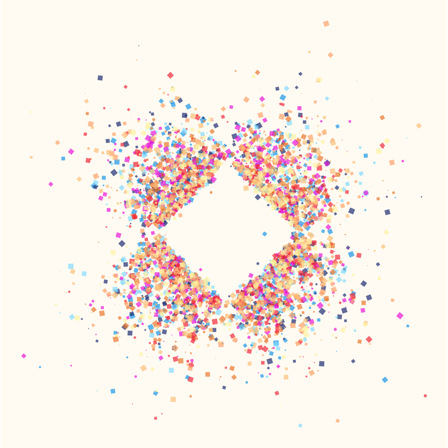
More shapes

The original algorithm was meant to look like dust particles floating away in the wind. In this iteration, we’ll do away with that restriction and add the ability to render our particles with any shape. I implemented this in two functions (why it has to be two is a weird reason…). If you want to render your points as different sized bubbles, you can use the bubbleize() function, and if you want to render them as polygons, you can use the regonize() function. Under the hood, these functions just add a few columns to your dataframe (r, angle, color) that we will use when plotting to render our points as polygons with geom_regon() from the ggforce package. Since I only want the points that move to be rendered as polygons, this function only applies these new fields to the moving points, and keeps the static points the same. It returns a list of two dataframes, one with the polygons and another with the static points.

More noise

From the beginning, I had hoped to incorporate flow fields to distort the moving particles, but in my first iteration I ran out of time to implement this idea. This time around, I caught a break, because I realized that Danielle Navarro’s wonderful jasmines package might have exactly what I needed. I ever so slightly adapted her unfold_tempest() function for my purposes, and it can now be used to apply some curl noise to the moving particles. The changes I’ve made include allowing you to specify between curl noise or Worley noise, and allowing for a variable scale parameter on each of the points being transformed. If you recall from last time, my particles have a concept of inertia, and now by adding a scale column to the points before passing it to unfold_tempest() you can make it such that points with smaller inertia are affected less. I typically do something like mutate(scale = inertia * 0.1).

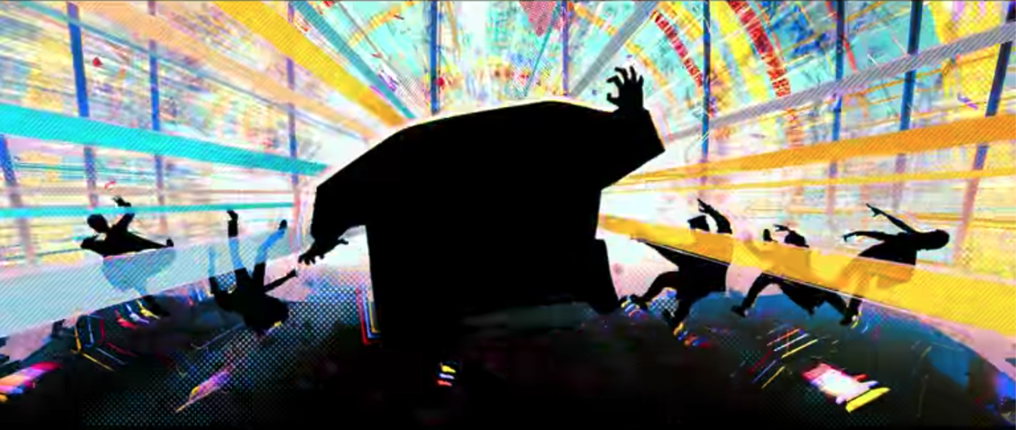
Into the Spider-Palettes

If you enjoyed the color palettes in this post so far, you can thank the incredible artists who worked on the best movie ever, Spider-Man: Into the Spider-Verse. When I was thinking of colors to use in this project, I thought it might be fun to sample palettes from the Spider-Verse. So, I went through the movie and picked several frames that I thought had great colors and sampled them to create some custom palettes. These are very much just my own interpretations, so take them as you will. Each is a list with the colors in a colors object, and one or more backgrounds named bg, bg2, bg3, etc...

A pipable system

One of my goals was to simplify the workflow for making art with this system by improving how “pipable” it is. There’s still a lot of parameters involved and it’s not easy to wrap your head around if you’ve never worked with it before, but I think I’ve streamlined the process of actually making these down to a few key steps. First, you define a seed for each shape—this will determine where your gaps are (ie, which points are static and which ones move). Next comes the meat of the algorithm: you generate a shape, split it according to your seed, apply a “gust” force in some direction, apply some noise with unfold_tempest(), and use regonize() to transform your points to polygons. To wrap up this post, here’s a couple of commented code examples, and as always, the code for the entire project can be found on my GitHub.

#Here I'll show how we can specify specific gaps on a line we generate and render the moving
#points as polygons
######################

#load libraries
#This assumes you've loaded all of the generic functions and palettes already
library(tidyverse)
library(EnvStats)
library(zoo)
library(ggforce)

#first we generate a seed with 10,000 points and we specify which points should
#move using the 'gaps' argument
seed1 <- gen_seed_line(data.frame(x = 0, xend = 100, y = 100, yend = 0),
                       n_grains = 10000, gaps = list(c(500, 1500), c(8000, 10000)))

#now we generate our dataframe for plotting
line1 <- 
  paint(data.frame(x = 0, xend = 100, y = 100, yend = 0), 10000) %>% #generate a line of points
  splitter(seed = seed1, wind_angle = 225) %>% #split that line according to our seed
  gust(angle = 225, force = 6, diff_mod = -0.01, inertia_mod = 0.017, jitter_min = 2, jitter_max = 20, jitter_mod = 0.4) %>% #apply a force at the angle of 225 degrees, using a negative diff_mod causes the points to spray somewhat outward
  mutate(scale = ifelse(inertia <= 2, 0, 0.1 * inertia)) %>% #add a scale value to each point based on its inertia so that points that move less will have less noise applied
  unfold_tempest(iterations = 70, type = "curl") %>% #apply curl noise to scatter points more
  regonize(min_r = 0.1, max_r = 2, pal = sunset$colors) #turn points that move into polygons and apply a palette

#when we plot we will plot the static points with geom_point, and the points that move with geom_regon
#we can tweak the color of the static points, as well as the number of sides of the polygons
#also note the background is set according to our palette
ggplot() +
  geom_point(data = line1$static, aes(x = x, y = y), alpha = 0.1, size = 0.1, color = "#FEFEFE") +
  geom_regon(data = line1$regons, aes(x0 = x, y0 = y, sides = 3, r = r, fill = color, angle = angle), alpha = 0.7, color = NA) +
  scale_fill_identity() +  
  scale_size_identity() +
  theme_void() +
  theme(panel.background = element_rect(fill = sunset$bg2, color = NA)) +
  coord_equal()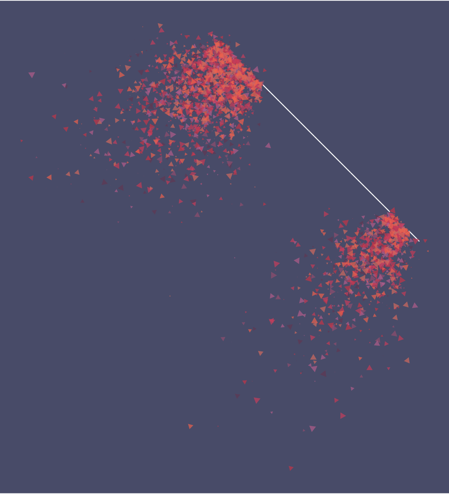

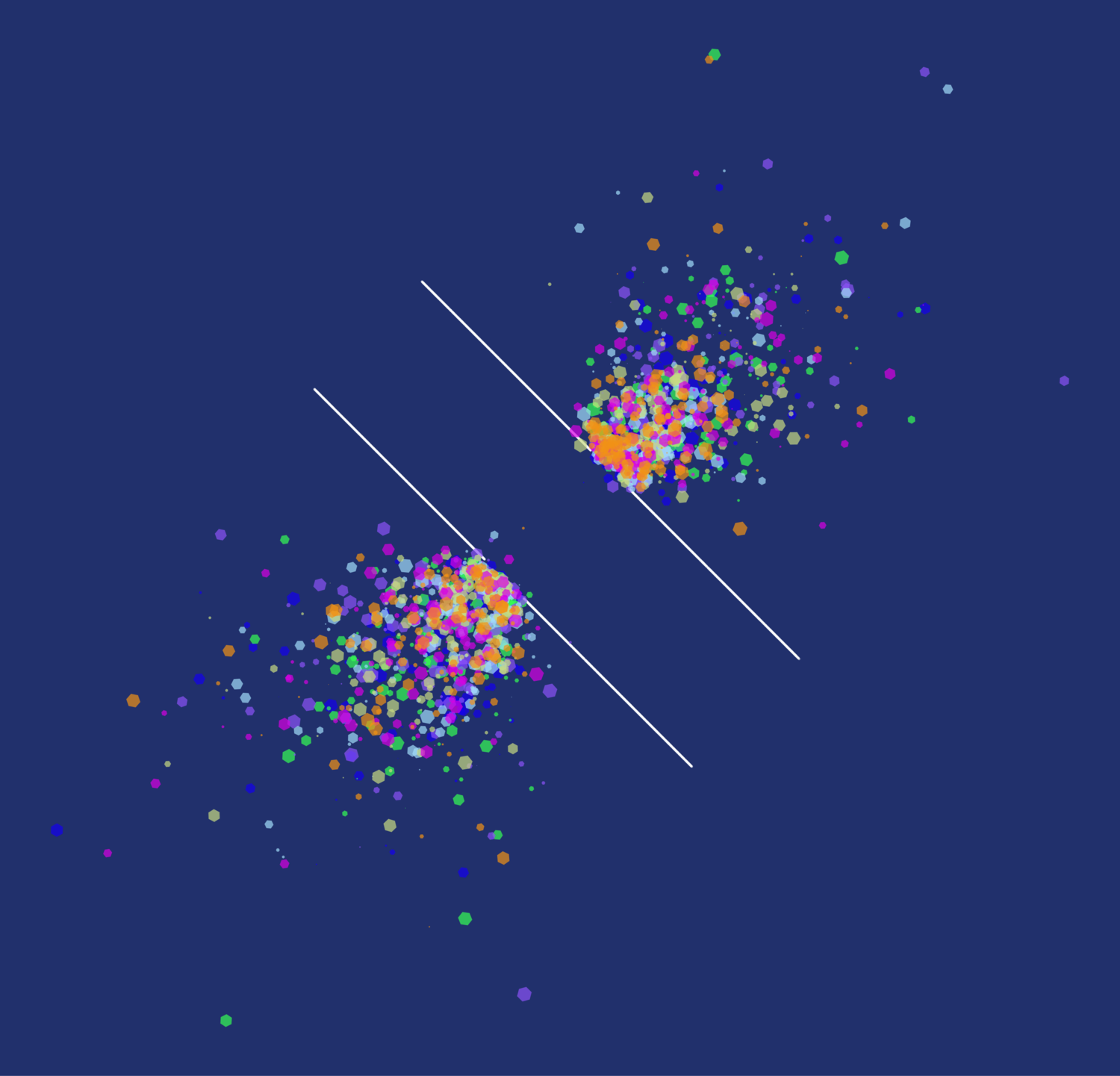
#Here I'll show how we can use some randomness and render a couple of circles
#using the 'bubbleize' function to render moving points as colored differently sized circles
######################

#load libraries
#This assumes you've loaded all of the generic functions and palettes already
library(tidyverse)
library(EnvStats)
library(zoo)
library(ggforce)

#set a random seed so that you can replicate the diagram if you like it
seed_rand <- sample(seq(0, 5000, by = 1), 1)
set.seed(seed_rand)

#set up random angles and centers for the circles
angle1 <- sample(0:360, 1)
angle2 <- sample(0:360, 1)
x0_1 <- sample(-50:50, 1)
x0_2 <- sample(-50:50, 1)
y0_1 <- sample(-50:50, 1)
y0_2 <- sample(-50:50, 1)

#generate two seeds using our random angles
#split_mod can be adjusted to get more or fewer gaps
seed1 <- gen_seed_cir(n_grains = 10000, r = 50, wind_angle = angle1, split_mod = 500)
seed2 <- gen_seed_cir(n_grains = 10000, r = 50, wind_angle = angle2, split_mod = 500)

#generate our first cirlce using the random angle1 and x0_1, y0_1
circle1 <- circle(points = 10000, r = 50, x0 = x0_1, y0 = y0_1) %>%
  splitter(seed = seed1, wind_angle = angle1) %>% #split circle by the seed
  gust(angle = angle1, force = 6, diff_mod = -0.01, inertia_mod = 0.017, jitter_min = 2, jitter_max = 20, jitter_mod = 0.4) %>% #apply force in the random angle direction
  mutate(scale = ifelse(inertia <= 2, 0, 0.1 * inertia)) %>% #add scale column
  unfold_tempest(iterations = 70, type = "curl") %>% #introduce curl noise to the points
  bubbleize(min_r = 0.5, max_r = 3, base_color = "#FEFEFE", pal = no_expectations$colors) #this sets the moving points as bubbles with different sizes, you can adjust min_r and max_r to adjust the size range

#do the same with the second circle
circle2 <- circle(points = 10000, r = 50, x0 = x0_2, y0 = y0_2) %>%
  splitter(seed = seed2, wind_angle = angle2) %>%
  gust(angle = angle2, force = 6, diff_mod = -0.01, inertia_mod = 0.017, jitter_min = 2, jitter_max = 20, jitter_mod = 0.4) %>%
  mutate(scale = ifelse(inertia <= 2, 0, 0.1 * inertia)) %>%
  unfold_tempest(iterations = 70, type = "curl") %>%
  bubbleize(min_r = 0.5, max_r = 3, base_color = "#FEFEFE", pal = no_expectations$colors)

#combine the two circles into one dataframe
circles <- rbind(circle1, circle2)

#plot the circles, this time just using geom_point
ggplot() +
  geom_point(data = circles, aes(x = x, y = y, size = size, color = color), alpha = 0.7) +
  scale_color_identity() +  
  scale_size_identity() +
  theme_void() +
  theme(panel.background = element_rect(fill = no_expectations$bg, color = NA)) +
  coord_equal()