Grid (12 Months of aRt, December)

September 13, 2020

It’s not December

Hi there, remember this? Way back in The Before Times I did this project called “12 Months of aRt”. I started in 2019 and did one generative art project per month, writing about them as I went. The thing is, I never finished. I got close, I finished 11 of the 12, and then things changed: I got busy, I lacked inspiration, the world got COVID, and… well, you get it. The point is, I’m finally here to finish things, even if it’s not on time. So please ignore the fact that the title says December and the publish date says September: just chalk it up to another anomaly in the alternate timeline that is 2020.

The inspiration

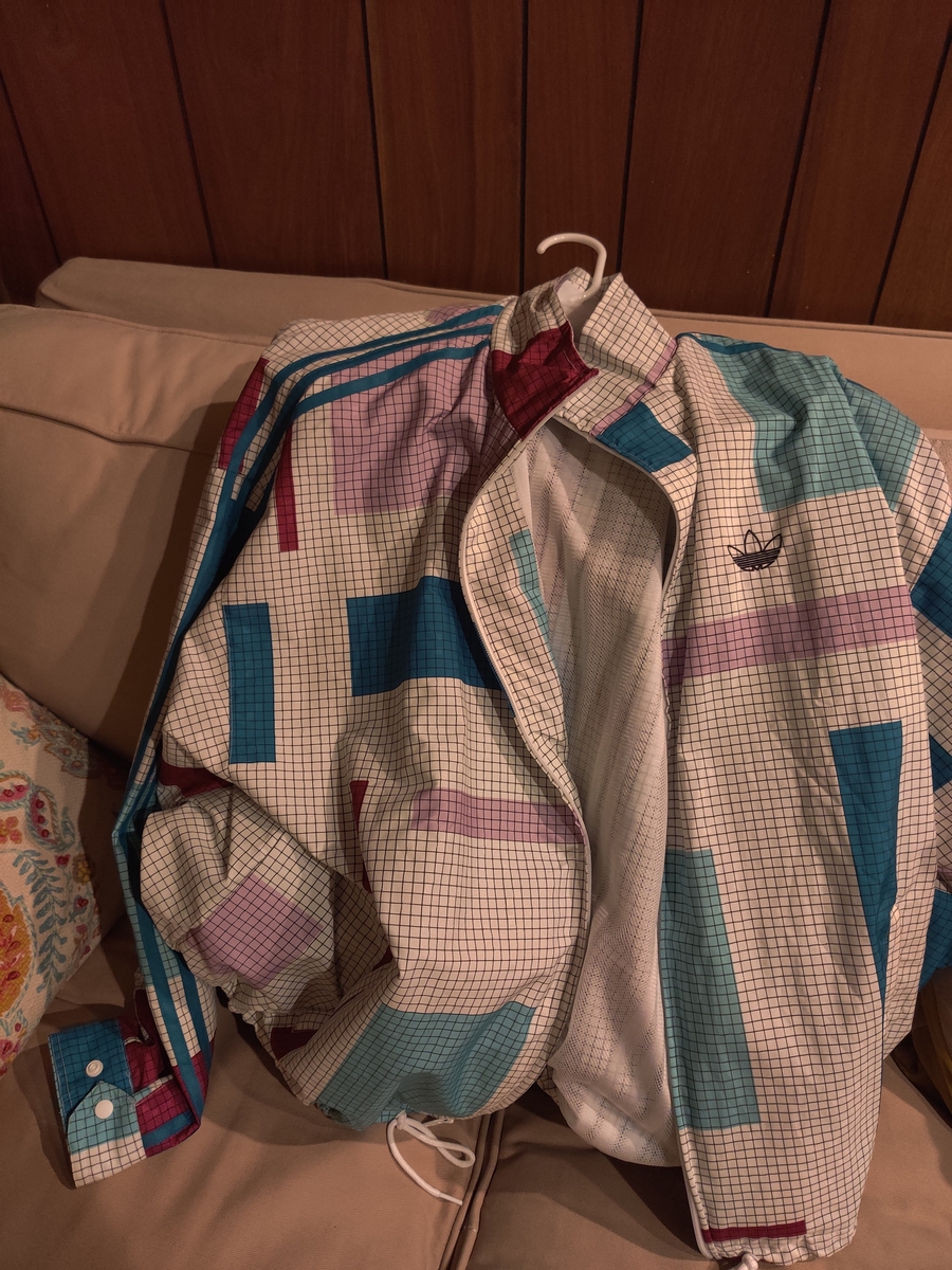
Sometimes inspiration comes from nature, other times from art, and in this case it came from fashion. I have this jacket from Adidas that has a design with a regular grid, overlaid with random looking rectangles. I don’t know if the design is generative, but it certainly has generative vibes and it immediately gave me an idea. I imagined a system based on two primary components: a grid and a set of polygons. The grid could be manipulated to have any number of rows or columns with different spacing and sizing, and the polygons could be any regular polygon (not just rectangles). The twist was that I would be able to distort the grid as it passed through the polygons.

The code

Let me begin by saying the code for this is unfinished. The system works and does what I want (mostly) but there are some known bugs, and several items on the to-do list for adding new features. That said, I think this is an excellent system to end my 12 Months of aRt project on, because it incorporates and remixes many techniques and pieces of code from previous projects.

building a grid

Unsurprisingly, the first step in our “grid” project is to construct a grid. Normally, in R, this is relatively easy with a function like expand.grid(), but that won’t suffice for our purposes. I wanted a grid that can have all sorts of different parameters: number of vertical lines, horizontal lines, different spacing between the lines, different start points and lengths, etc. Most importantly, I wanted each line in the grid to have many points so that the distortions we apply later can have a smooth appearance.

This function definitely has some bugs if you don’t set the parameters in a specific way, but it still works. The general idea is as follows: based on the input parameters like number of lines, gap between the lines, and length, it produces a dataframe with a set of many points that represent those lines by making a set of start and endpoints for each line and then doing a linear interpolation between those points. One important concept from here is the linear interpolation or lerp function. Many programming languages implement their own version of this, but since R doesn’t, we can make a simple version of our own.

#interpolates points along a line
#provide the x,y of the start and endpoints, and the number of points to interpolate
lerp <- function(start_x, start_y, end_x, end_y, points) {
  tibble(id = 1:points) %>%
    mutate(d = id / points,
           x = (1 - d) * start_x + d * end_x,
           y = (1 - d) * start_y + d * end_y)
}

With our grid function in hand, we can make all sorts of combinations of lines, like this:

my_grid <- 
  grid_gen(h_lines = 50, h_gap = 3, h_points = 200, h_ystart = 0,
           v_lines = 50, v_gap = 3, v_points = 200, v_xstart = 0)

ggplot() +
  geom_path(data = new_grid$grid, aes(x = x, y = y, group = line), size = 0.4)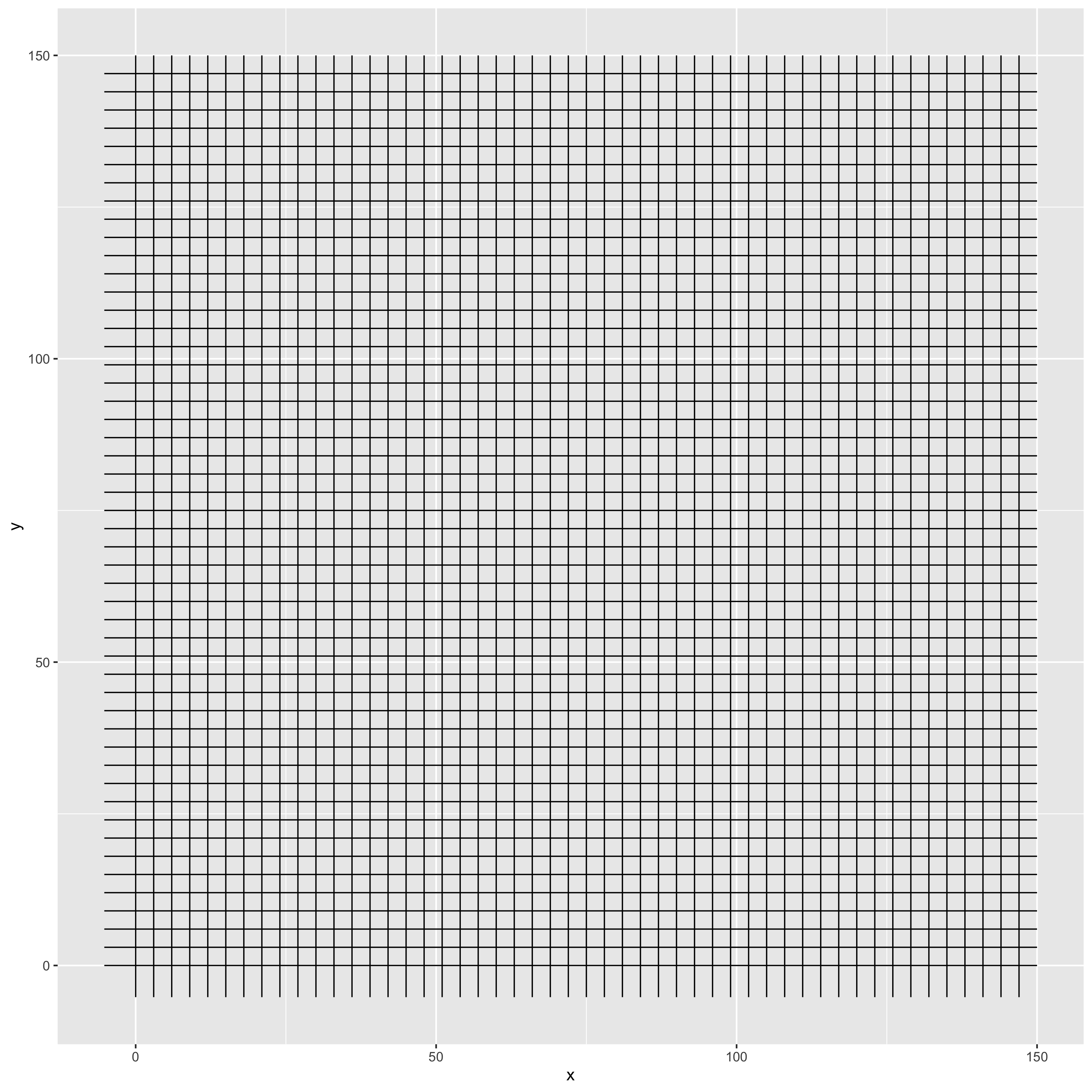

Adding polygons

The other main ingredient of our system is random polygons that can be overlaid on our grid. There’s two primary functions here: one for rectangles and another for regular polygons. Why two? Because I wanted the rectangles to vary in width and height, and that goes against the regular part of regular polygon. Both of these functions look very similar, so I’ll just go through the polygon function. The idea here is that you have lots of options: you can specify parameters yourself (things like number of polygons, how many edges each polygon has, their locations, size, etc.) or you can leave those arguments NULL and the function will randomize it for you. I’ve already made a function that takes in the location, edges, radius, etc. and constructs a regular polygon, so to make a bunch of them, I use a familiar pattern of putting all my randomized parameters in a dataframe, then using rowwise() and mutate() to run my gen_regon() function across each row, generating the polygons. The final step is to remove overlapping polygons (if you want), using some code that Dewey Dunnington generously donated.

grid_regons <- function(grid, n = NULL, edges = NULL, cx = NULL, cy = NULL, r = NULL, color = NULL, overlap = FALSE) {
  #randomize and set up parameters 
  if(is.null(n)) {n <- sample(3:15, 1)}
  if(is.null(edges)) {
    edges <- sample(3:8, n, replace = TRUE)
  } else if(length(edges) == 1) {
    edges <- rep(edges, n)
  }
  if(is.null(cx)) {
    cx <- sample(seq(grid$bounds[1], grid$bounds[3], by = 0.1), n, replace = TRUE)
  }
  if(is.null(cy)) {
    cy <- sample(seq(grid$bounds[4], grid$bounds[2], by = 0.1), n, replace = TRUE)
  }
  if(is.null(r)) {
    r <- rpareto(n, location = sample(seq(max(grid$bounds) / 20, max(grid$bounds) / 10, by = 0.1), 1), shape = sample(3:4, 1))
  }
  if(is.null(color)) {
    colors <- c("#666666")
  } else {
    colors <- color
  }
  
  regons <- 
    tibble(edges = edges, cx = cx, cy = cy, r = r) %>%
    rowwise() %>%
    mutate(data = list(gen_regon(cx = cx, cy = cy, edges = edges, r = r, start_angle = ifelse(edges %% 2 == 0, 180 / edges, 90))))
  
  if(!overlap) {
    regons_list <- 
      bind_rows(regons$data, .id = "id") %>%
      remove_overlaps()
    
    regons_df <- 
      regons_list$polygons %>%
      group_by(id) %>%
      mutate(color = sample(colors, 1, replace = TRUE))
  } else {
    regons_df <- bind_rows(regons$data, .id = "id") %>%
      group_by(id) %>%
      mutate(color = sample(colors, 1, replace = TRUE))
  }
  
  grid$regons <- regons_df 
  if(!overlap) {
    grid$centroids <- regons_list$centroids
  }
  return(grid)
}

Distortions

The final piece of our puzzle is distorting our grid as it passes through the polygons. Before we get into the actual distortion, one bit of business: to decide which points will get distorted, we need to know which points on our grid are inside of our polygons. I have some plans to expand upon this system, so for reasons of future-proofing, this point-in-polygon detection lives inside of a function called assign_inertia(). I’ve talked about the concept of inertia before, and I’ve covered point-in-polygon detection as well, so for now just trust me that before you apply a distortion, you need to run assign_inertia() on your grid/polygon data.

For our first distortion, I implemented a flow field using an adaptation of Danielle Navarro’s unfold_tempest() function. I’ve covered this previously in my “dust” system, so I won’t go into much detail here. Just know that you can pipe your data into this function and it will create a distortion based on curl noise. You can adjust the noise using the iterations and scale parameters. A distorted grid might look like this:

data <- 
  grid_gen(h_lines = 150, h_gap = 0.15, h_points = 800,
           v_lines = 150, v_gap = 0.15, v_points = 800) %>%
  grid_rects(n = 30, color = neon1) %>%
  assign_inertia() %>%
  unfold_tempest(iterations = 8, scale = 0.01, type = "curl")

ggplot() +
  geom_path(data = data$grid, aes(x = x, y = y, group = line), size = 0.2) +
  geom_polygon(data = data$rects, aes(x = x, y = y, group = id, fill = color), alpha = 0.7) +
  scale_fill_identity() +
  theme_void()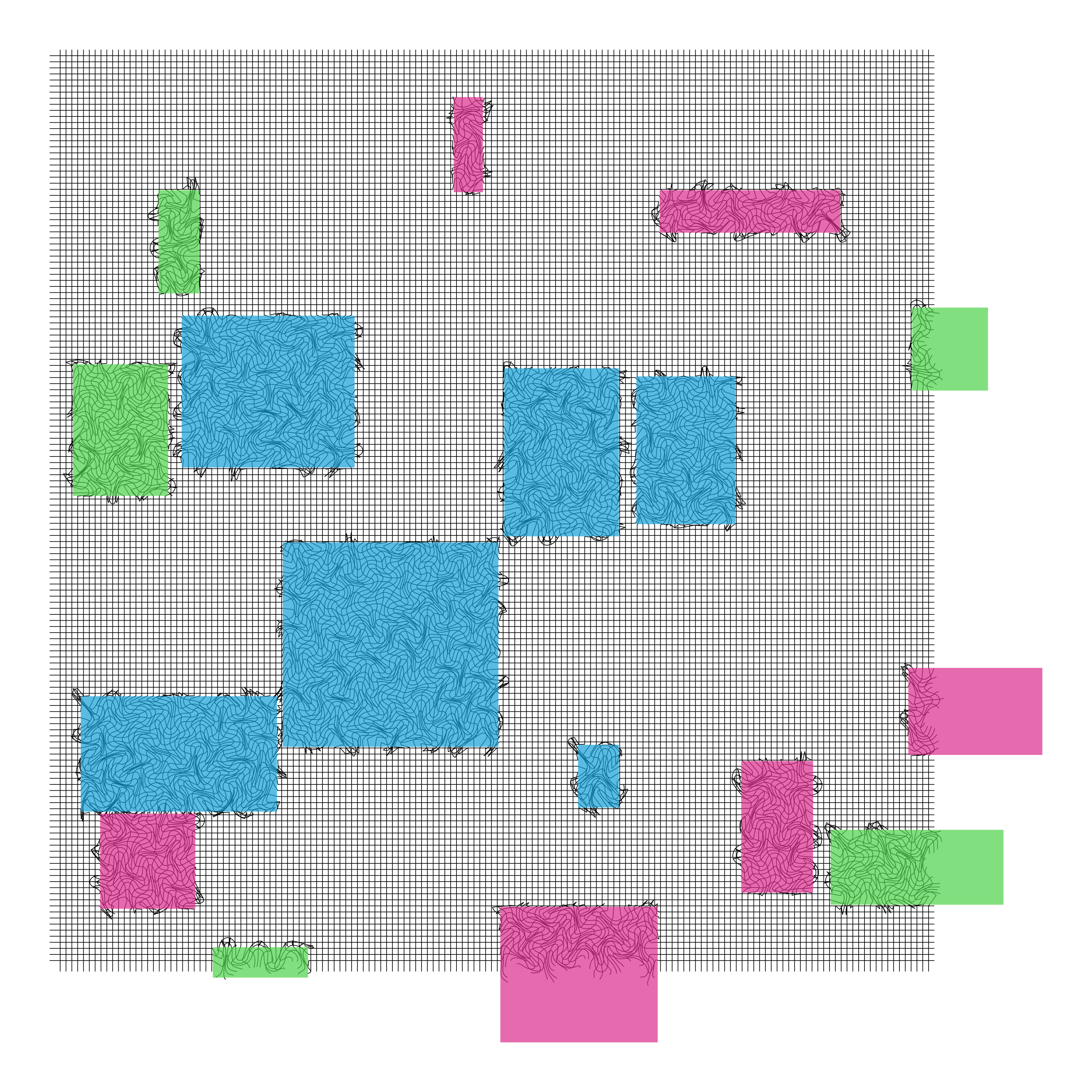

The final bit I added to this system was a lens distortion. I got the original idea from looking at pictures made with a fisheye lens, and you might know the distortion by that name, but it turns out that type of effect is generally called a barrel distortion. Researching how to apply this type of distortion led me down a total rabbit hole into math and photography forums. It turns out there’s a lot of ways to do this, and it’s quite a big problem in the optics field. You can find many different models of lens distortion, unfortunately most of the implementations I found were ways to correct it, and what I want to do is the opposite. After some tinkering I finally got the math right (at least I think I did), and the nice thing about this method is that you can adjust the parameters to apply either a barrel distortion, or a pincushion distortion.

grid_distort <- function(grid, k, k2) {
  grid_in <- grid$grid %>% filter(inout)
  grid_out <- grid$grid %>% filter(!inout)
  
  distorted <- 
    grid_in %>%
    mutate(x_rescale = x - centroid_x,
           y_rescale = y - centroid_y,
           ru_2 = x_rescale^2 + y_rescale^2,
           x_d = x_rescale * (1 + (k * ru_2) + (k2 * ru_2^2)),
           y_d = y_rescale * (1 + (k * ru_2) + (k2 * ru_2^2)),
           x_distort = x_d + centroid_x,
           y_distort = y_d + centroid_y
    ) %>%
    select(line, id, d, x = x_distort, y = y_distort, line_direction, inout, polygon_id, centroid_x, centroid_y, inertia)
  
  
  grid_distort <- rbind(grid_out, distorted) %>% arrange(id)
  grid$grid <- grid_distort
  return(grid)
}

A quick breakdown of this function: we take the grid and separate it into the points that are inside the polygons and those that are outside. We take the points that are inside, rescale them so that the centroid of the polygon is (0, 0), then apply the equation for lens distortion using the supplied parameters k and k2. If the lens parameters are negative it will produce a barrel distortion, if positive it will give a pincushion distortion. This function could definitely be improved by providing an easier way to set the parameters. Currently it relies on a lot of guessing and checking, as they only produce a sensible distortion in quite a narrow range that depends on the size of the grid and polygons. A couple of examples:

#barrel distortion with circles
data <- 
  grid_gen(h_lines = 200, h_gap = 2, h_points = 200, h_ystart = 0, h_xstart = 0, h_xend = 400) %>%
  grid_regons(n = 30, edges = 200, color = neon2) %>%
  assign_inertia() %>%
  grid_distort(k = -0.00000005, k2 = -0.00000005)

ggplot() +
  geom_path(data = data$grid, aes(x = x, y = y, group = line), size = 0.3) +
  geom_polygon(data = data$regons, aes(x = x, y = y, group = id, fill = color), alpha = 0.7) +
  scale_fill_identity() +
  theme_void()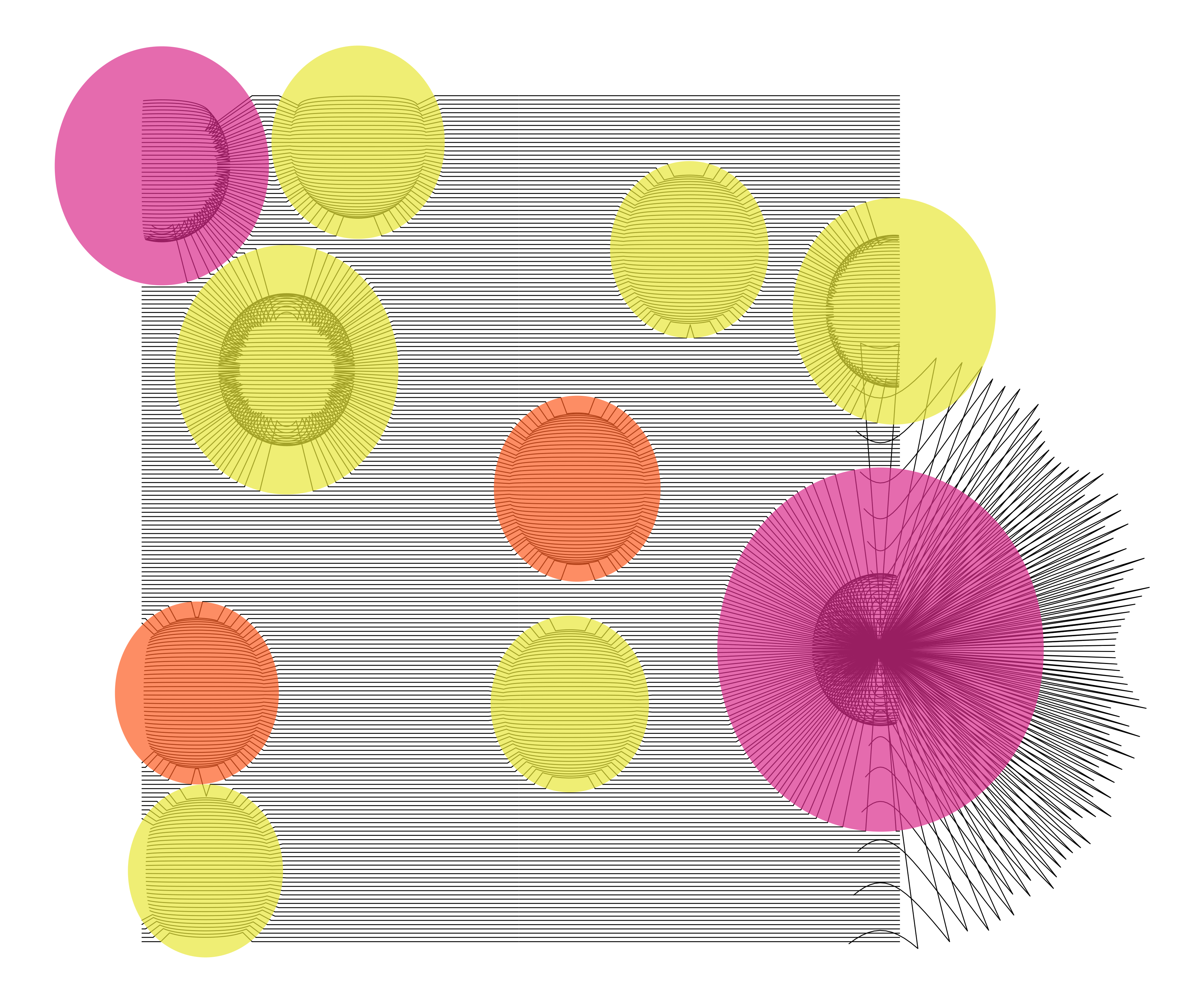

#pincushion distortion with random polygons
data <- 
  grid_gen(h_lines = 150, h_gap = 2, h_points = 200, h_ystart = 0, h_xstart = 0, h_xend = 200,
           v_lines = 80, v_gap = 1, v_points = 200, v_xstart = 150, v_ystart = 50, v_yend = 500) %>%
  grid_regons(n = 10, color = neon2) %>%
  assign_inertia() %>%
  grid_distort(k = 0.00000005, k2 = 0.00000005)

ggplot() +
  geom_path(data = data$grid, aes(x = x, y = y, group = line), size = 0.3) +
  geom_polygon(data = data$regons, aes(x = x, y = y, group = id, fill = color), alpha = 0.7) +
  scale_fill_identity() +
  theme_void()

These images clearly show another issue with this function: it allows the distortions to escape the polygon boundary. I don’t necessarily mind this all the time, it can be an interesting effect, but I do have plans to implement a clip parameter so that I can choose if I want to clip things to the polygon boundary or not.

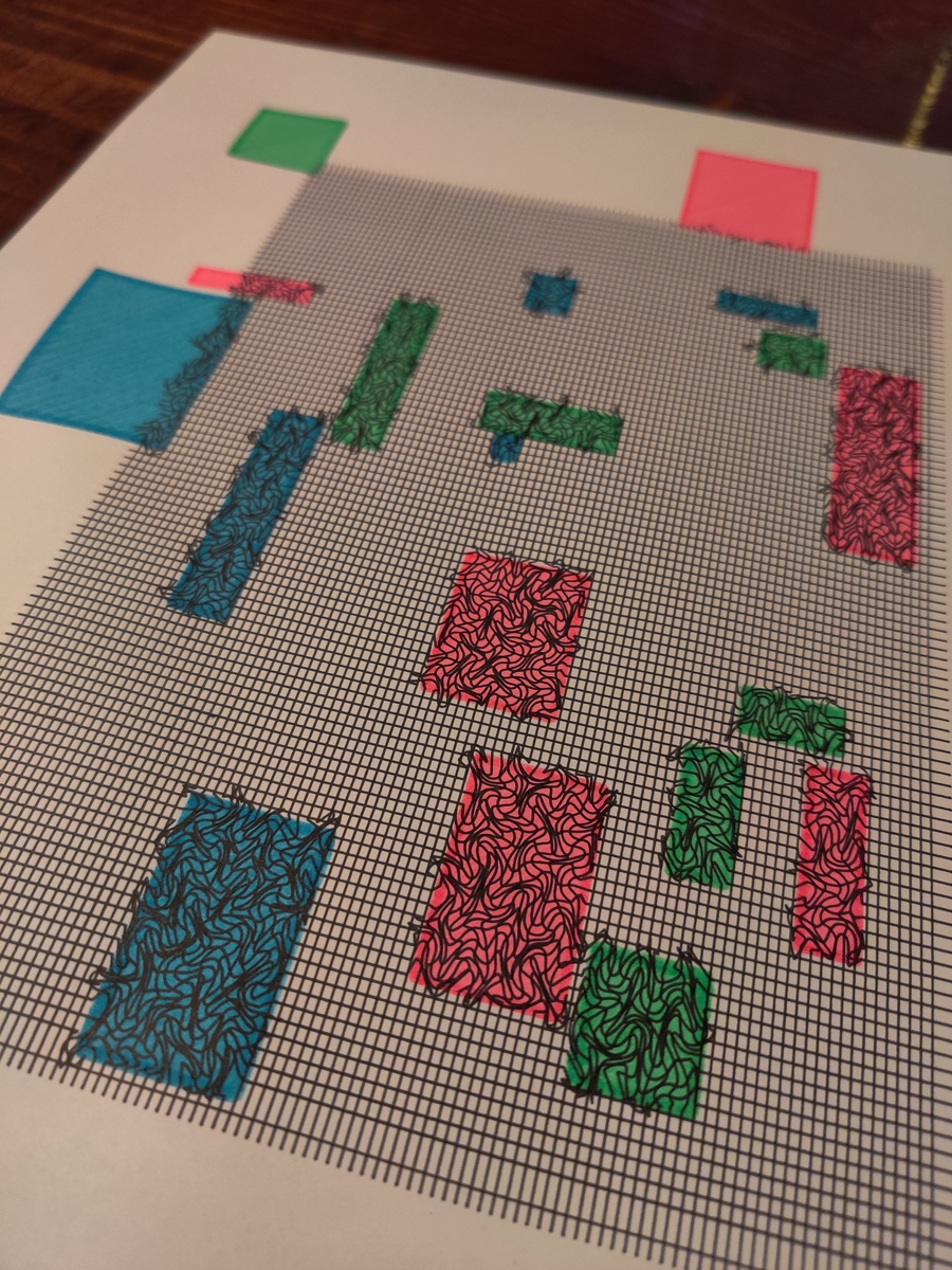
Making aRt physical

The colors for these pieces were not chosen randomly, they were chosen to match the Windsor and Newton Neon Promarkers, because from the beginning, this one was bound for my pen plotter. Perhaps the most exciting development in the R generative art world in 2020 was the fawkes package, that allows you to interface with the AxiDraw pen plotter directly from R. I had been lusting after an AxiDraw for a while and the development of fawkes was the kick I needed to finally hit the order button. Unfortunately, when I first got my plotter, I had no good place to put it (it literally sat on the uneven floor next to my desk for weeks), then I went to visit my parents for a couple months, so the plotter has seen almost 0 use since I bought it. That all changes now.

I plan to produce a bunch of pen plots from this system, but for now enjoy this small test I did with some rectangles and flow field distortion:

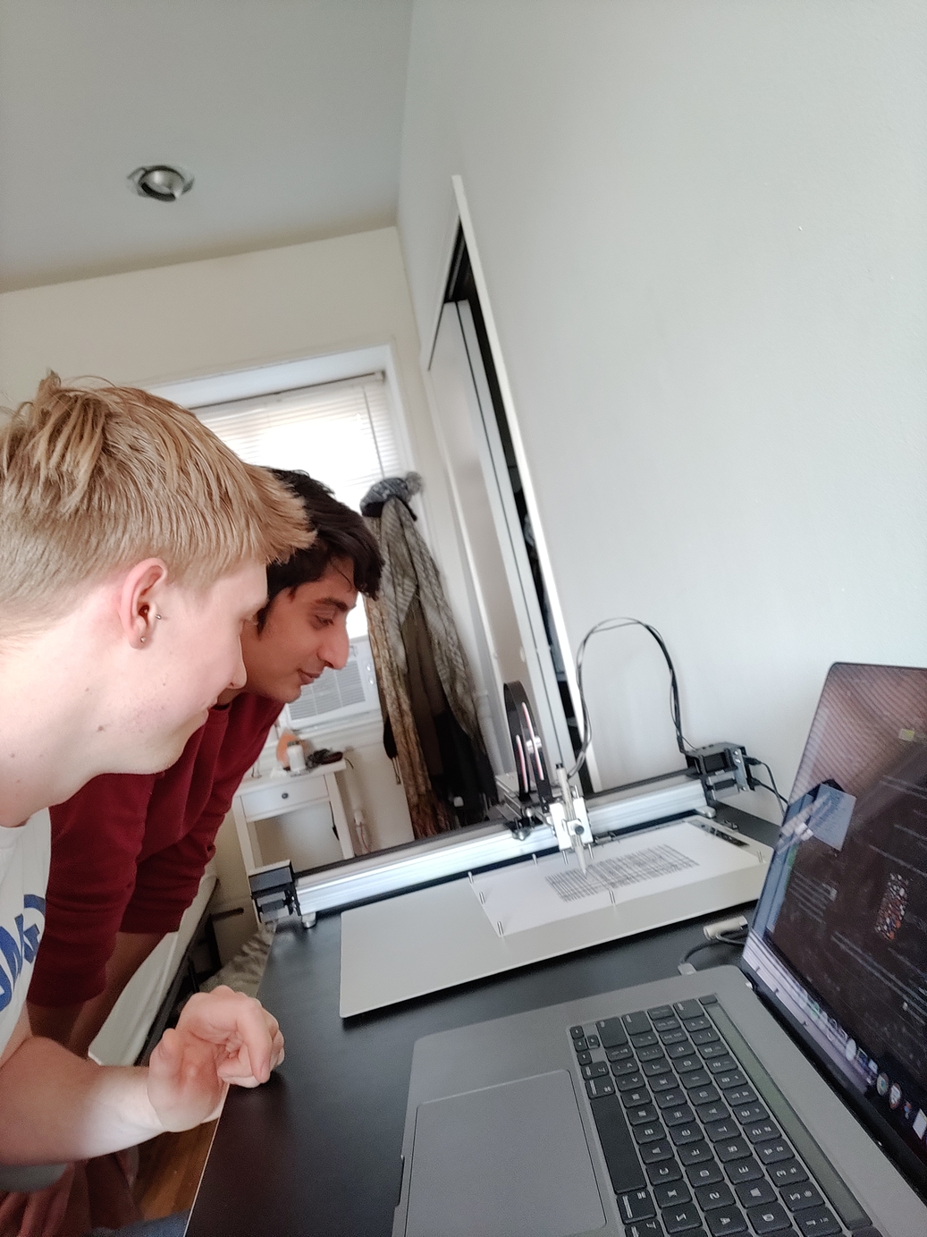
Watching the plotter work is completely mesmerizing, so much so that as I was plotting this my partner stopped his work, came upstairs, and we both just stared at it for a good 5 minutes.

The end of 12 Months of aRt

This post will be the last of 12 Months of aRt. I will continue to make generative art, but there will be no schedule and fewer blogs in the future. I like the outputs of this project to varying degrees: some of them I’d be proud to hang on my wall, and others just seem like fun experiments. But overall I’m immensely satisfied to have finished this project, and it has been one of the most rewarding things I’ve done over the last couple years. I’ve learned so much about math, programming, and design through this process, and I hope to write (or speak) more about that some day. Perhaps the most rewarding part has been seeing others inspired by my work. Every so often someone posts their aRt on Twitter and mentions my blog as inspiration, and every one of those posts makes me smile. I sincerely hope you’ve enjoyed reading about this process and following along as I ventured into the world of generative art. And I hope you’ll keep up with my work (perhaps through my newsletter), I promise there’s more exciting things to come!